Overview

Questions

• How do you create appealing plots in Python?

• How do you compare distributions of data?

• How do different plotting libraries work?

Objectives

• Examples of seaborn for Python.

• Make box plots, violin plots, and histograms in seaborn.

• Some examples of plots using bokeh and ggplot.

Plotting with seaborn

Python has powerful built-in plotting capabilities and for this exercise, we will focus on using the seaborn package, which facilitates the creation of highly-informative plots of structured data. The seaborn library is built on matplotlib and features very nice color palettes. This library makes manipulating the features of a matplotlib plot somewhat easier. For an introduction to this package, see the seaborn documentation.

To install the package, use conda:

$ conda install seaborn

For this exercise, we will use a different data file, called “surveys_complete.csv”, containing all the complete data observations from the plot surveys used in previous lessons. Download this file from the course repository or pull the all new changes from the repository if you haven’t done so already.

Getting Started

Create a new Jupyter notebook for this lesson and begin by importing the Pandas package and seaborn. We also need to import the matplotlib plotting functions pyplot in order to directly call any of the plotting functions for matplotlib

import pandas as pd
import matplotlib.pyplot as plt
import seaborn as sns

Here, we have given seaborn the alias sns.

Now load the DataFrame:

surveys_complete = pd.read_csv('surveys_complete.csv', index_col=0)

For this exercise, we will use a different version of the ecological dataset from our previous lessons. This version has only the complete observations, without missing entries for any of the columns. There are also a few additional columns providing information about the taxonomy of the species collected and the type of plot/enclosure.

A Simple Scatterplot

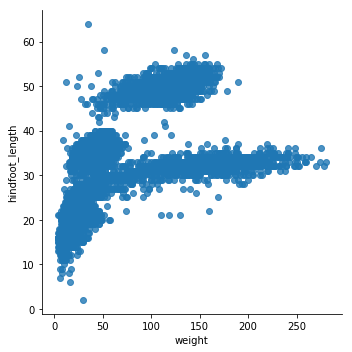
Let’s start with a basic scatterplot. We’ll simply plot the weight on the horizontal axis and the hind foot length on the vertical axis. This uses the seaborn function .lmplot(). This function can take a Pandas DataFrame directly. It also will fit a regression line, by default. Since we may not want to visualize these data with a regression line, we will use the fit_reg=False argument.

sns.lmplot(x="weight", y="hindfoot_length", data=surveys_complete, fit_reg=False)

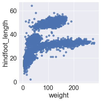
Out of the box, seaborn will plot with a given set of aesthetics. We may want to change the label font size and make the background gray. For this, we can call the .set() method. If this method is called without any arguments, sns.set(), this will switch on the seaborn defaults, which changes the background color to gray and overlays white grid lines (i.e., a similar background to ggplot2 in R). We can add an argument to also change the font size for all of our downstream figures:

sns.set(font_scale=1.5)

This will increase the font size of the labels by 50% in all of our subsequent plots.

sns.lmplot(x="weight", y="hindfoot_length", data=surveys_complete, fit_reg=False)

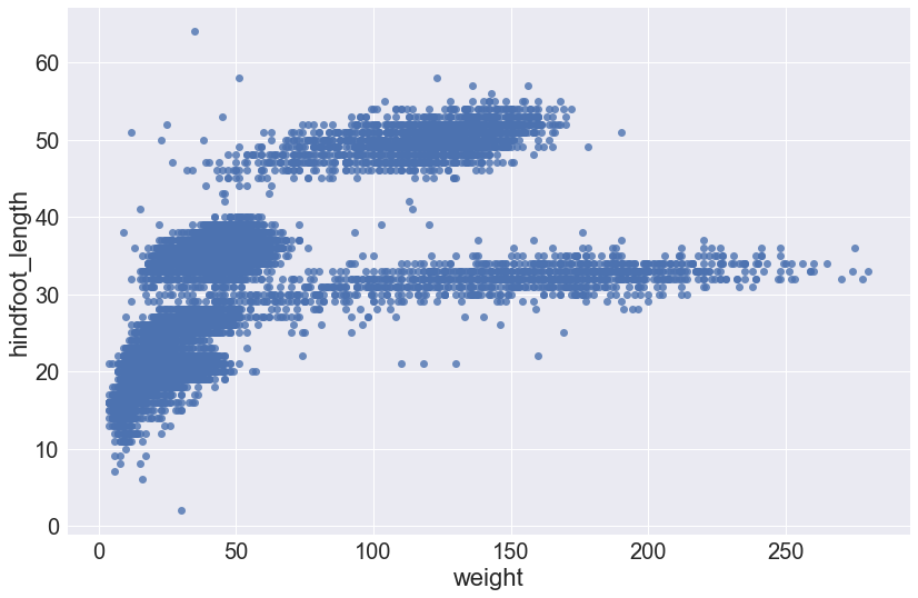
The plot size is small, by default, and with seaborn, there isn’t a way to change the size of every plot with a single function. Further, this is done differently depending on the plot function we use because some functions return matplotlib objects and others are drawn using a grid object.

For .lmplot(), we can set the plot size directly as arguments in the function call using the size and aspect arguments. These arguments control the height and width of the object, respectively.

sns.lmplot(x="weight", y="hindfoot_length", data=surveys_complete, fit_reg=False, height=8, aspect=1.5)

Changing marker aesthetics

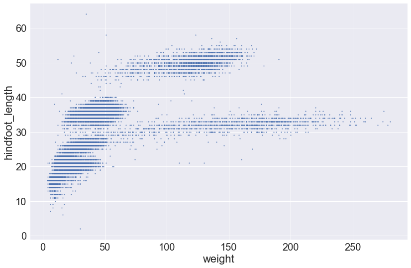
One issue with this plot is that because we have a large dataset, it is difficult to adequately visualize the points on our graph. This is called “overplotting”. One way to avoid this is to change the size of the marker. Here we use the argument scatter_kws that takes a dictionary of keywords and values that are passed to the matplotlib scatter function.

sns.lmplot(x="weight", y="hindfoot_length", data=surveys_complete, fit_reg=False, height=8, aspect=1.5, scatter_kws={"s": 5})

Alternatively, we can change the marker type using the markers keyword argument. By default, lmplot() sets markers='8'. If we want to change the marker, we must use the correct matplotlib code. Let’s change the markers to X-es:

sns.lmplot(x="weight", y="hindfoot_length", data=surveys_complete, fit_reg=False, height=8, aspect=1.5, markers='x')

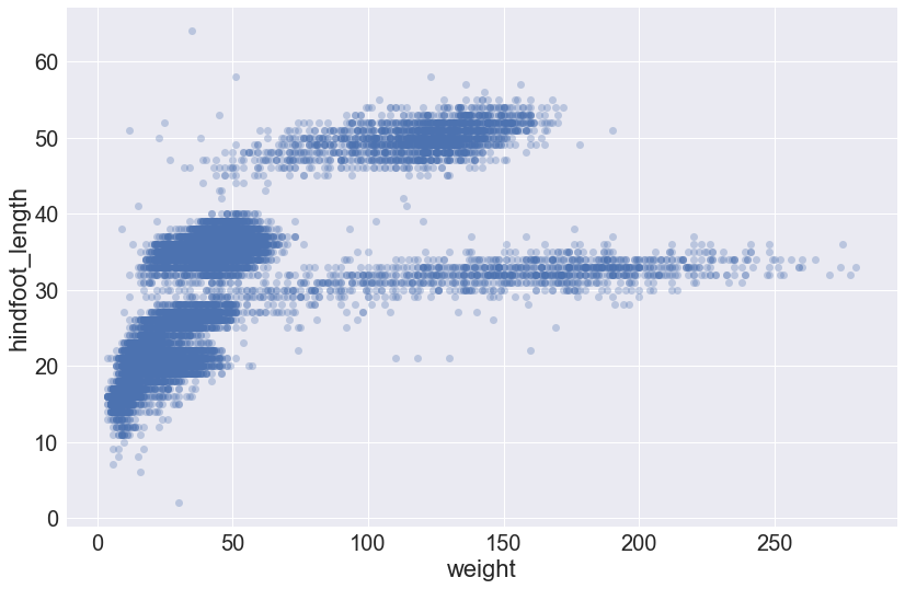
Another way to avoid overplotting is to use transparency so that regions of the plot with many points are darker. This is achieved using the scatter_kws argument and setting the alpha value. (This is using alpha compositing.)

sns.lmplot(x="weight", y="hindfoot_length", data=surveys_complete, fit_reg=False, height=8, aspect=1.5, scatter_kws={'alpha':0.3})

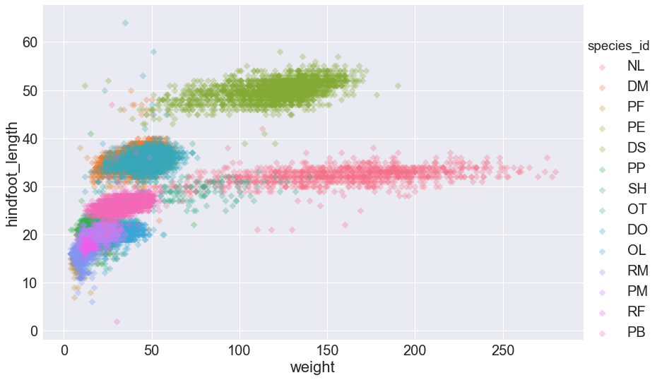
Coloring markers by a categorical value

We can also specify that the species_id labels indicate categories that determine a point’s color:

sns.lmplot(x="weight", y="hindfoot_length", data=surveys_complete, 
           fit_reg=False, height=8, aspect=1.5, scatter_kws={'alpha':0.3,"s": 50}, 
           hue='species_id', markers='D')

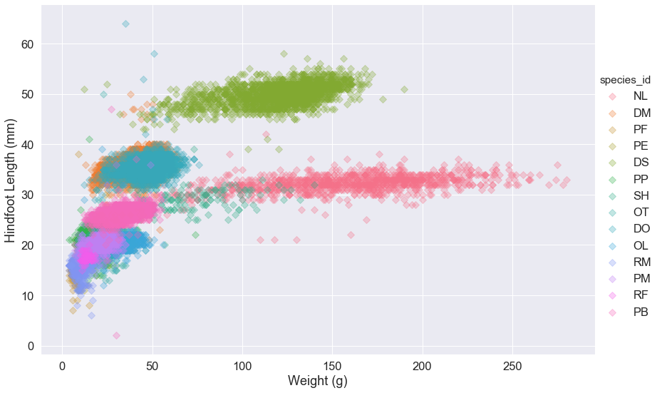
Setting the axis labels

There are different ways to set figure properties using seaborn. For .lmplot(), we can create a figure variable and use a member method of that variable to set the axis labels.

my_fig = sns.lmplot(x="weight", y="hindfoot_length", data=surveys_complete, 
                    fit_reg=False, height=8, aspect=1.5, 
                    scatter_kws={'alpha':0.3,"s": 50}, 
                    hue='species_id', markers='D')
my_fig.set_axis_labels('Weight (g)', 'Hindfoot Length (mm)')

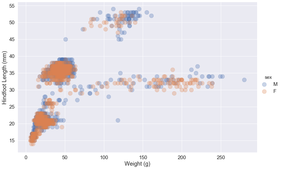
Scatter plot for a single plot

How would you plot the hind foot length and weight for just a single plot? Remember how to access subsets of a DataFrame based on conditional criteria? Plot the scatter plot above for only plot number 12 and color by sex. (Make the markers larger circles.)

Solution

my_fig = sns.lmplot(x="weight", y="hindfoot_length", 
                    data=surveys_complete[surveys_complete.plot_id == 12], 
                    fit_reg=False, height=8, aspect=1.5, 
                    scatter_kws={'alpha':0.3,"s": 200}, 
                    hue='sex', markers='8')
my_fig.set_axis_labels('Weight (g)', 'Hindfoot Length (mm)')

Box Plots & Violin Plots

We often like to compare the distributions of values across different categorical variables. Box plots and violin plots are often used to do this in a simple way.

In seaborn, both the .boxplot() and .violinplot() functions return matplotlib Axes objects. Thus, these plot functions do not have arguments for height and aspect like the scatter plot function above.

In order to change the size of these plots, we must create a matplotlib figure and axes and set the dimensions of the figure. First, let’s decide on the figure size we will use for the rest of our seaborn plots.

We can put these dimensions into a tuple variable called plot_dims.

plot_dims = (14, 9)

Now, every time we create a new plot that returns a matplotlib Axes object, we can call the .subplots() function to change some of the aesthetics. Because of the iteritve way in which figures are built using matplotlib, we need to always execute our creation of the figure and the plot function in a single notebook cell.

fig, ax = plt.subplots(figsize=plot_dims)
sns.boxplot(x='species_id', y='hindfoot_length', data=surveys_complete)
ax.set(xlabel='Species ID', ylabel='Hindfoot Length (mm)')

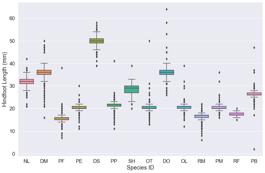
Note that for the .boxplot() function, we can simply set the x and y values by giving the column names from our DataFrame. Then we must use the data=surveys_complete argument to indicate our DataFrame object.

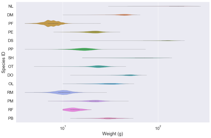
Now let’s use a violin plot to visualize the weight data. For these data, we would also like the weight to be on the log10 scale. We will make this plot horizontal, so we’ll set the horizontal axis to be on the log scale. An easy way to do this is to create a new graph variable from our .violinplot() function and then call the .set_xscale() that is a member method of the graph variable.

fig, ax = plt.subplots(figsize=plot_dims)
g = sns.violinplot(x='weight', y='species_id', data=surveys_complete, 
                   linewidth=0.2, orient="h", cut=0)
g.set_xscale('log', base=10)
ax.set(ylabel='Species ID', xlabel='Weight (g)')

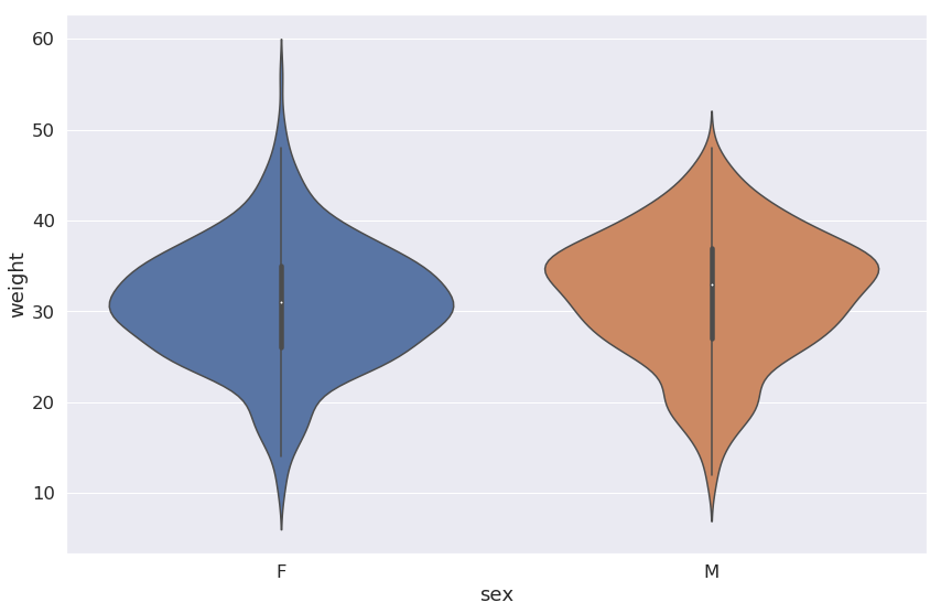
Violin plot for a single species

Use seaborn to make a violin plot comparing the relative distributions of weight measurements for different sexed animals from a single species, Onychomys leucogaster (OL), one of the coolest rodent species:

Solution

fig, ax = plt.subplots(figsize=plot_dims)
sns.violinplot(x='sex', y='weight', data=surveys_complete[surveys_complete.species_id == 'OL'])

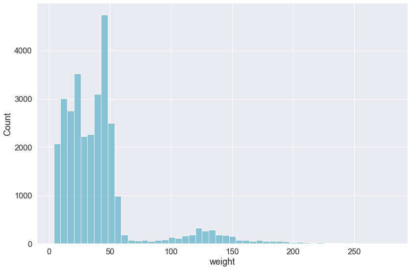
Histograms

Often, a histogram is a better way to visualize a distribution. This is relatively simple using seaborn’s .displot() function. This function does not take a Pandas DataFrame, but can take a Pandas Series (i.e., column in our DataFrame). This function also can take come other arguments like color, which takes values that specify the color of histogram based on matplotlib’s colors. We will make our plot cyan using the 'c' color code. Additionally, we will specify bins=50 so that our histogram is not plotted using too many or too few bins.

sns.displot(surveys_complete['weight'], color='c',bins=50, 
            height=8, aspect=1.5)

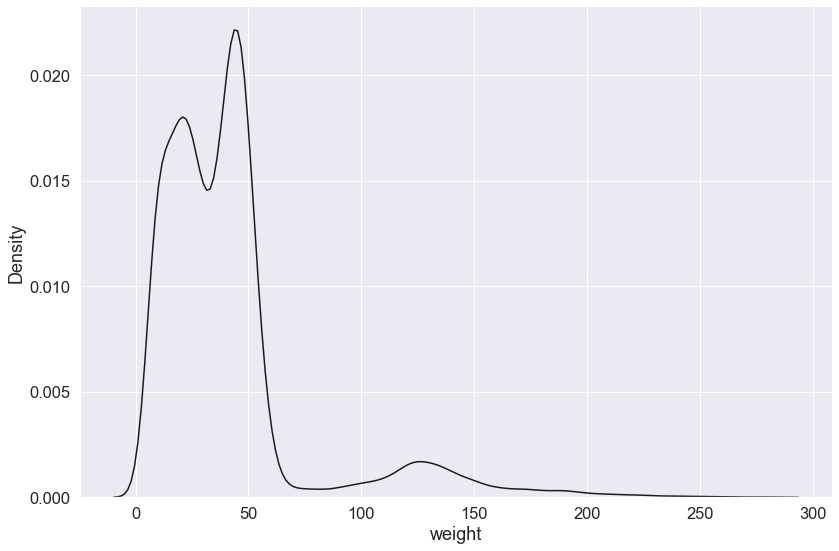
By default, the .displot() function plots the density as a histogram, alternatively, you can plot a kernel density estimate by setting the kind argument to kind="kde" (the default is kind="hist") and removing the bins argument.

sns.displot(surveys_complete['weight'], color='k', kind="kde", 
            height=8, aspect=1.5)

Plotting with bokeh

Another library called bokeh can create amazing, interactive graphics using D3.js (javascript). This package is also easy to install with conda:

$ conda install bokeh

Return to your Jupyter notebook and import the necessary bokeh plotting tools:

from bokeh.plotting import figure 
from bokeh.io import output_notebook, show

Here we are importing functions to create a figure and to output that figure to our Jupyter notebook.

We can now execute the output_notebook() function that will ensure that our Javascript images are displayed in our html notebook.

output_notebook()

This figure also uses the histogram function from numpy. So we have to first import that package:

import numpy as np

We can reproduce the histogram of the weights of all our observations.

hist, edges = np.histogram(surveys_complete['weight'], density=True, bins=100)
my_fig = figure(title="Weight (g)",background_fill_color="#EBC8EB")
my_fig.quad(top=hist, bottom=0, left=edges[:-1], right=edges[1:],fill_color="#036564", line_color="#033649")
show(my_fig)

We can also save this file as an html file that we can share with others or embed in files on the web. To do this, we need to include some other bokeh functions:

from bokeh.resources import CDN
from bokeh.embed import file_html

And create an html object and save it to a file using standard Python file i/o:

html = file_html(my_fig, CDN, "Weight Histogram")
out = open('weight_hist_bokeh.html','w')
out.write(html)
out.close()

If you open the file you created in your web browser, you now have an interactive version of your figure. You can then use this to embed in a website.

Take-Home Challenge: More Visualizations in Python

Continue to use seaborn and bokeh to try out different visualizations.

1. Produce a histogram of the hindfoot length for only the species observed in the genus Peromyscus. Note that this particular dataset includes a column called "genus". So you can subset out only the entries for Peromyscus individuals. Try making the histogram using both seaborn and bokeh. Consider altering the bin numbers to help visualize the distribution.

2. This dataset also has a column called "plot_type". That says what kind of plot in which the animal was captured. The different plot types are specific experimental set-ups for this kind of study. Create a visualization that helps us better understand how the species ("species_id") might be influenced by the plot type. For example, are some species prevented from entering certain plot types?

Solutions

The solutions will be posted in 4 days. Feel free to use the #scripting_help channel in Slack to discuss these exercises.

Key Points

• There are many tools for plotting in Python.