EEOB/BCB 5460: Programming with Python
Working With Pandas DataFrames in Python
Overview
Questions
How do you import data into Python?
How do you create a DataFrame and access its contents?
How do you create simple plots?
Objectives
Describe the Python Data Analysis Library (Pandas).
Load Pandas.
Use
read_csvto read tabular data into Python.Describe what a DataFrame is in Python.
Access and summarize data stored in a DataFrame.
Define indexing as it relates to data structures.
Perform basic mathematical operations and summary statistics on data in a Pandas DataFrame.
Create simple plots.
Starting with Data
We can automate much of our research workflow using Python. It’s efficient to spend time building the code to perform these tasks because once it is built, we can use it over and over on different datasets that use a similar format. This makes our methods easy to reproduce and easy to adapt to new projects. We can also share our code with colleagues and they can replicate the same analysis.
Getting Set Up
To help the lesson run smoothly, let’s ensure everyone is in the same directory.
This should help us avoid path and file name issues. At this time please
navigate to the directory containing the course repository on your computer.
Before starting, be sure to pull the most recent changes from the repository using git pull origin master.
If you’re working in Jupyter Notebook be sure
that you start your notebook in the course-files/python directory. If you do not have this directory, please see the instructions in the Setup page.
You will want to use a Jupyter notebook or the Spyder IDE console to run this lesson. Both of these tools make it easy to view in-line plots.
To start a new Python session in a Jupyter notebook:
$ cd course-files/python
$ jupyter notebook
This typically brings up your default web browser and opens the Jupyter home screen.
Select New->Python 3. Name this session 03-starting-wtih-data.
Note that you can also start a Jupyter notebook from the Anaconda Navigator launch screen. This will likely open the notebook in your home directory and you can then navigate through your file system to get to the course-files/python directory.
Alternatively, you can start a Spyder instance and navigate to the course-files/python directory from the console using Unix commands.
Our Data
For this lesson, we will be using the Portal Teaching data, a subset of the data from the ecological study by Ernst et al. (2009): Long-term monitoring and experimental manipulation of a Chihuahuan Desert ecosystem near Portal, Arizona, USA Specifically, we will be using files from the Portal Project Teaching Database.
- This section will use the
surveys.csvfile that can be downloaded from thecourse-files/pythonfolder of the course repository. Pull from the course repository and change to tocourse-files/pythonor copy thesurveys.csvfile to the directory from which you would like to work.
In this lesson, we are studying the species and weight of (vertebrate) animals captured in plots in our study
area. The observed data are stored as a .csv file (comma-separated value): each row holds information for a
single animal, and the columns represent:
| Column | Description |
|---|---|
| record_id | Unique id for the observation |
| month | month of observation |
| day | day of observation |
| year | year of observation |
| plot_id | ID of a particular plot |
| species_id | 2-letter code |
| sex | sex of animal (“M”, “F”) |
| hindfoot_length | length of the hindfoot in mm |
| weight | weight of the animal in grams |
The first few rows of our first file look like this:
record_id,month,day,year,plot_id,species_id,sex,hindfoot_length,weight
1,7,16,1977,2,NL,M,32,
2,7,16,1977,3,NL,M,33,
3,7,16,1977,2,DM,F,37,
4,7,16,1977,7,DM,M,36,
5,7,16,1977,3,DM,M,35,
6,7,16,1977,1,PF,M,14,
7,7,16,1977,2,PE,F,,
8,7,16,1977,1,DM,M,37,
9,7,16,1977,1,DM,F,34,
Pandas in Python
One of the best options for working with tabular data in Python is to use the Python Data Analysis Library (a.k.a. Pandas). The Pandas library provides data structures, produces high quality plots with matplotlib and integrates nicely with other libraries that use NumPy (which is another Python library) arrays.
Python does not load all available libraries by default. We have to
add an import statement to our code in order to use library functions. To import
a library, we use the syntax import libraryName. If we want to give the
library a nickname to shorten the command, we can add as myNickName.
Import the pandas library using the common nickname pd is below.
import pandas as pd
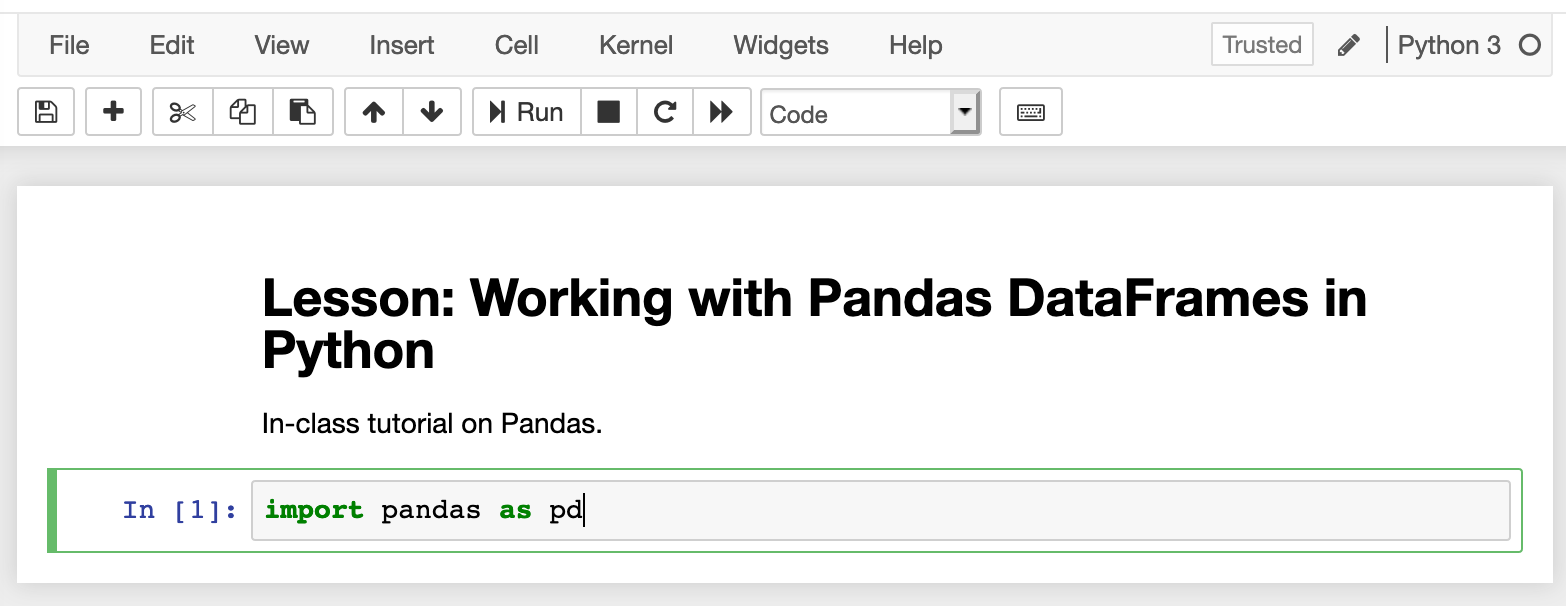
If you’re using a Jupyter notebook for this lesson, it should look like this:
Remember that the import pandas as pd syntax means that we have given the alias pd to the pandas library. Thus, we don’t have to use the whole name when we invoke pandas functions.
Documenting Code
Let’s take a moment to talk about proper documentation again. One major benefit of using Jupyter Notebooks is that it gives us a way to provide clear and descriptive comments about our code. This is a good place to write a description of this notebook.
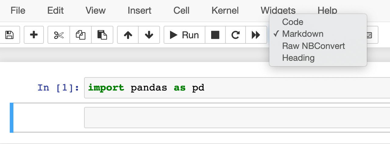
Add a new cell in your notebook and change the cell type to Markdown.
You can also use the arrow buttons to move this cell to the top of your notebook.
Now we can write a description of this notebook using Markdown.
# Lesson: Working with Pandas DataFrames in Python

In-class tutorial on Pandas.
Reading CSV Data Using Pandas
We will begin by locating and reading our survey data which are in CSV format.
We can use Pandas’ read_csv function to pull the file directly into a
DataFrame.
What’s a DataFrame?
A DataFrame is a 2-dimensional data structure that can store data of different
types (including characters, integers, floating point values, factors and more)
in columns. It is similar to a spreadsheet or an SQL table or the data.frame in
R. A DataFrame always has an index (0-based). An index refers to the position of
an element in the data structure.
pd.read_csv("surveys.csv")
       record_id  month  day  year  plot_id species_id  sex  hindfoot_length  \
0              1      7   16  1977        2         NL    M             32.0
1              2      7   16  1977        3         NL    M             33.0
2              3      7   16  1977        2         DM    F             37.0
3              4      7   16  1977        7         DM    M             36.0
4              5      7   16  1977        3         DM    M             35.0
5              6      7   16  1977        1         PF    M             14.0
6              7      7   16  1977        2         PE    F              NaN
7              8      7   16  1977        1         DM    M             37.0
...          ...    ...  ...   ...      ...        ...   ...             ...
35547      35548     12   31  2002        7         DO    M             36.0
35548      35549     12   31  2002        5        NaN  NaN              NaN

       weight
0         NaN
1         NaN
2         NaN
3         NaN
4         NaN
5         NaN
6         NaN
7         NaN
...       ...
35547    51.0
35548     NaN

[35549 rows x 9 columns]
We can see that there were 33,549 rows parsed into a DataFrame. Each row has 9 columns. The first column is the index of the DataFrame. The index is used to identify the position of the data, but it is not an actual column of the DataFrame (it is not labeled).
It looks like the read_csv function in Pandas read our file properly. However, we haven’t saved any data to memory, and we cannot work with it until we do that.
We need to assign the DataFrame to a variable.
Remember that a variable is a name for a value, such as x,
or data. We can create a new object with a variable name by assigning a value to it using the = operator.
Let’s call the imported survey data surveys_df:
surveys_df = pd.read_csv("surveys.csv")
Notice when you assign the imported DataFrame to a variable, Python does not
produce any output on the screen. We can print the value of the surveys_df
object by typing its name into the Python command prompt. This will print the data frame just like above.
surveys_df
Inspecting Our Species Survey DataFrame
Now we can start working with our data. First, let’s check the data type of the
data stored in surveys_df using the type function. The type function and
__class__ attribute tell us that surveys_df is <class 'pandas.core.frame.DataFrame'>.
type(surveys_df)
pandas.core.frame.DataFrame
The output is the same if you use this:
surveys_df.__class__
pandas.core.frame.DataFrame
We can also enter surveys_df.dtypes at our prompt to view the data type for each
column in our DataFrame. int64 represents numeric integer values - int64 cells
cannot store decimals. object represents strings (letters and numbers). float64
represents numbers with decimals.
surveys_df.dtypes
record_id            int64
month                int64
day                  int64
year                 int64
plot_id              int64
species_id          object
sex                 object
hindfoot_length    float64
weight             float64
dtype: object
Useful Ways to View DataFrame objects in Python
There are multiple methods that can be used to summarize and access the data
stored in DataFrames. Note that we call the method by using
the object or method name surveys_df.object or surveys_df.method(). So surveys_df.columns provides an index
of all of the column names in our DataFrame.
Querying DataFrames
There are several methods that allow you to inspect your DataFrame.
Print the column names:
surveys_df.columnsPrint the first
4lines of the DataFramesurveys_df.head(4)Print the last
4lines of the DataFramesurveys_df.tail(4)Print the dimensions of the DataFrame
surveys_df.shape
Summarizing Data in a Pandas DataFrame
We’ve read our data into Python. Next, let’s perform some quick summaries of the DataFrame to learn more about the data that we’re working with. We might want to know how many animals were collected in each plot, or how many of each species were caught. We can summarize different aspects of our data using groups. But first we need to figure out what we want to group by.
Let’s begin by exploring our data and view the column names:
surveys_df.columns
Index(['record_id', 'month', 'day', 'year', 'plot_id', 'species_id', 'sex',
       'hindfoot_length', 'weight'], dtype=object)
Let’s get a list of all the species. The pd.unique method tells us all of
the unique values in the species_id column. These are two-character identifiers of the species names (e.g., NL represents the rodent Neotoma albigula).
pd.unique(surveys_df['species_id'])
array(['NL', 'DM', 'PF', 'PE', 'DS', 'PP', 'SH', 'OT', 'DO', 'OX', 'SS',
       'OL', 'RM', nan, 'SA', 'PM', 'AH', 'DX', 'AB', 'CB', 'CM', 'CQ',
       'RF', 'PC', 'PG', 'PH', 'PU', 'CV', 'UR', 'UP', 'ZL', 'UL', 'CS',
       'SC', 'BA', 'SF', 'RO', 'AS', 'SO', 'PI', 'ST', 'CU', 'SU', 'RX',
       'PB', 'PL', 'PX', 'CT', 'US'], dtype=object)
How many plots were recorded for this dataset?
Create a list of unique plot ID’s found in the surveys data. Call it
plot_names. How many unique plots are there in the data?Is there a simpler solution for doing this?
Solution
# 1
plot_names = list(pd.unique(surveys_df['plot_id']))
print(len(plot_names))

# 2
print(surveys_df['plot_id'].nunique())
Note that the
.nunique()method does not count null (i.e.,nan) values.
Groups in Pandas
We often want to calculate summary statistics grouped by subsets or attributes within fields of our data. For example, we might want to calculate the average weight of all individuals per plot.
We can calculate basic statistics for all records in a single column using the
.describe() method:
surveys_df['weight'].describe()
count    32283.000000
mean        42.672428
std         36.631259
min          4.000000
25%         20.000000
50%         37.000000
75%         48.000000
max        280.000000
Name: weight, dtype: float64
We can also extract one specific metric if we wish:
Like the lowest weight
surveys_df['weight'].min()
4.0
The maximum weight
surveys_df['weight'].max()
280.0
The mean of the weight column
surveys_df['weight'].mean()
42.672428212991356
The standard deviation of the weight
surveys_df['weight'].std()
36.63125947458399
Count the number of observations made for weight:
surveys_df['weight'].count()
32283
But if we want to summarize by one or more variables, for example the weight for each sex, we need to
use the Pandas DataFrame .groupby() method. Once we’ve created a re-orgaized DataFrame, we
can quickly calculate summary statistics by a group of our choice.
Group data by the sex of each observed individual:
sorted_data = surveys_df.groupby('sex')
The method .describe() will return descriptive stats including: mean,
median, max, min, std and count for a particular column in the data. Pandas’
.describe() method will only return summary values for columns containing
numeric data.
With the sorted data, we can obtain the summary statistics for the weight column separated by sex.
sorted_data['weight'].describe()
       count       mean        std  min   25%   50%   75%    max
sex
F    15303.0  42.170555  36.847958  4.0  20.0  34.0  46.0  274.0
M    16879.0  42.995379  36.184981  4.0  20.0  39.0  49.0  280.0
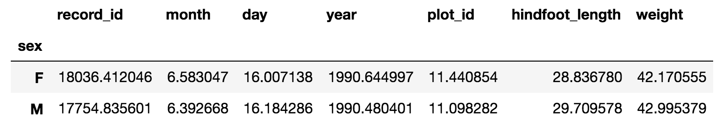
We can also get the mean for each numeric-valued column, grouped by sex:
sorted_data.mean()
The .groupby() method is powerful in that it allows us to quickly generate
summaries of categorical data.
How many individuals were recorded as female and how many were male?
Using the
.describe()method on the DataFrame sorted by sex, determine how many individuals were observed for each.Solution
Female = 15690
Male = 17348
Group by two columns
What happens when you group by two columns and then view mean values:
- Hint: you can use a list in the arguments of the
.groupby()method,['plot_id','sex']Solution
sorted_data2 = surveys_df.groupby(['plot_id','sex'])
sorted_data2.mean()
Summarize a single column
Summarize weight values for each plot in your data.
Solution
by_plot = surveys_df.groupby('plot_id')
by_plot['weight'].describe()
Quickly Creating Summary Counts in Pandas
Let’s next count the number of samples for each species. We can do this in a few
ways, but we’ll use groupby combined with a count() method.
species_counts = surveys_df.groupby('species_id')['record_id'].count()
species_counts
species_id
AB      303
AH      437
AS        2
BA       46
CB       50
CM       13
CQ       16
...
Or, we can also count just the rows that have the species “PL” (Peromyscus leucopus):
surveys_df.groupby('species_id')['record_id'].count()['PL']
36
Basic Math Functions
If we wanted to, we could perform math on an entire column of our data. For example let’s multiply all weight values by 2. A more practical use of this might be to normalize the data according to a mean, area, or some other value calculated from our data.
Multiply all weight values by 2 and store values in a Pandas object called double_weight:
double_weight = surveys_df['weight'] * 2
If we summarize double_weight, then the summary will indicate that these values are twice the original weights:
double_weight.describe()
count    32283.000000
mean        85.344856
std         73.262519
min          8.000000
25%         40.000000
50%         74.000000
75%         96.000000
max        560.000000
Name: weight, dtype: float64
Quick & Easy Plotting Using Pandas
We can plot our summary stats using Pandas, too.
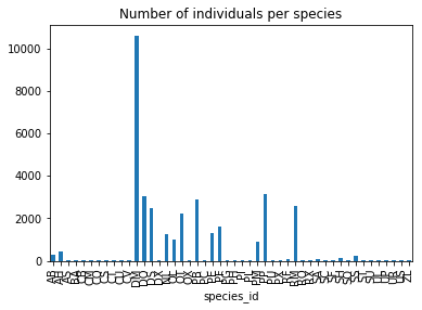
Now, we can make a quick bar chart of the species counts
species_counts.plot(kind='bar',title='Number of individuals per species')
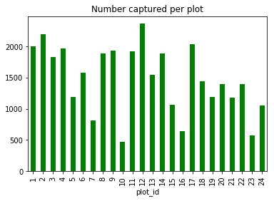
We can also look at how many animals were captured in each plot:
total_count = surveys_df.groupby('plot_id')['record_id'].nunique()
And plot a bar chart describing the number of individuals captured at each plot. Also, let’s make it so that all of the bars are colored green.
total_count.plot(kind='bar',title='Number captured per plot', color='green')
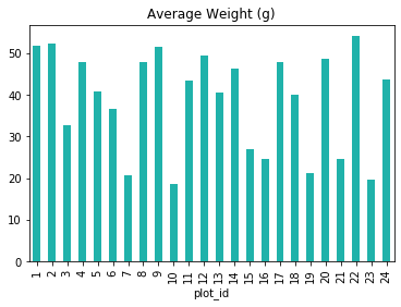
Plot the average weight across all species in each plot
Create a bar plot that shows the average weight of all of the animals captured in that plot. Also, choose an interesting or pleasing color from the list of named web colors.
Solution
plot_weight_means = surveys_df.groupby('plot_id')['weight'].mean()
plot_weight_means.plot(kind='bar',title='Average Weight (g)',color='LightSeaGreen')
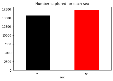
Plot the number of females and the number of males in the dataset
Create a bar plot that shows the total number of each sex captured for the entire dataset.
Solution
counts_by_sex = surveys_df['record_id'].groupby(surveys_df['sex']).count()
counts_by_sex.plot(kind='bar',title='Number captured for each sex',color=['k', 'r'])
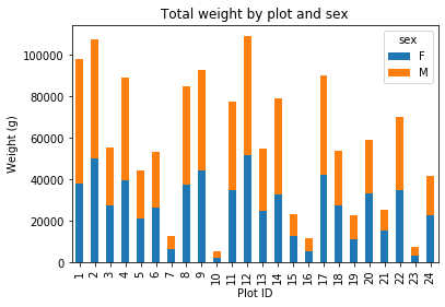
More Fun with Plotting
Now we will plot something a little bit more difficult. We will use a stacked bar plot to show how both weight and sex are distributed across each plot in the study.
First we group data by plot and by sex, and then calculate a total for each plot.
by_plot_sex = surveys_df.groupby(['plot_id','sex'])
plot_sex_count = by_plot_sex['weight'].sum()
plot_sex_count
This calculates the sums of weights for each sex within each plot as a table
plot  sex
plot_id  sex
1        F      38253
         M      59979
2        F      50144
         M      57250
3        F      27251
         M      28253
4        F      39796
         M      49377
...
Then we’ll use .unstack() on our grouped data to figure out the total weight that each sex contributed to each plot.
plot_sex_count.unstack()
sex            F        M
plot_id
1        38253.0  59979.0
2        50144.0  57250.0
3        27251.0  28253.0
4        39796.0  49377.0
5        21143.0  23326.0
6        26210.0  27245.0
7         6522.0   6422.0
...
Now, create a stacked bar plot with those data where the weights for each sex are stacked by plot.
spc = plot_sex_count.unstack()
s_plot = spc.plot(kind='bar',stacked=True,title="Total weight by plot and sex")
s_plot.set_ylabel("Weight (g)")
s_plot.set_xlabel("Plot")
Take-Home Challenge: More Fun with DataFrames and Plotting
Continue working with the
surveys_dfDataFrame on the following challenges:
Plot the average weight over all species and plots sampled each year (i.e., year on the horizontal axis and average weight on the vertical axis).
Come up with another way to view and/or summarize the observations in this dataset. What do you learn from this?
Solutions
The solutions will be posted in a few days. Feel free to use the
#scripting_helpchannel in Slack to discuss these exercises.
Key Points
Python can be used to work with complex data structures.
Pandas is a powerful tool for dealing with tabular data.
You can easily summarize data.
There are ways to readily visualize summaries.