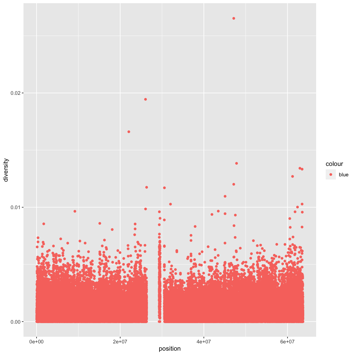
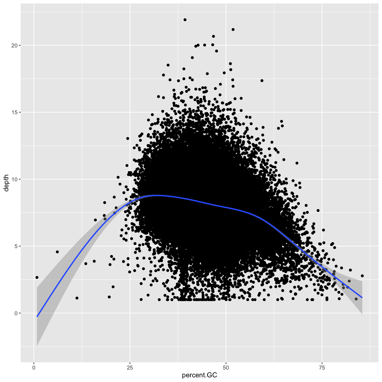
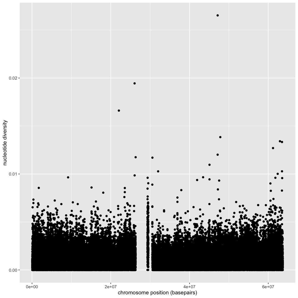
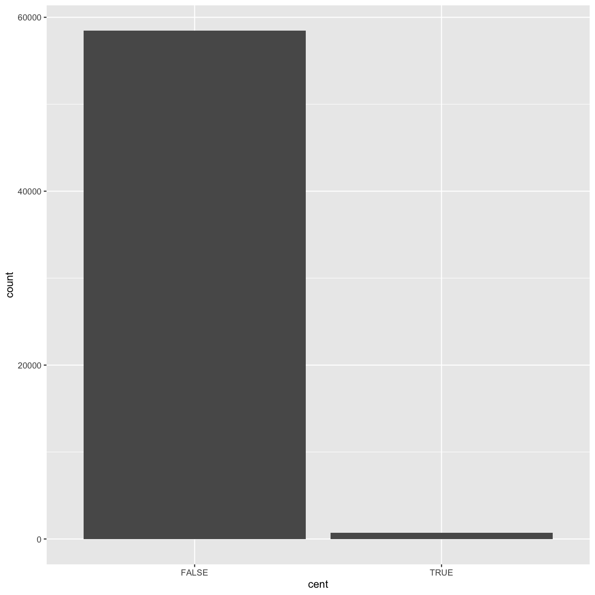
Getting Started with R and RStudio
Overview
Teaching: 20 min
Exercises: 10 minQuestions
How to find your way around RStudio?
How to start and organize a new project from RStudio
How to put the new project under version control and integrate with GitHub?
Objectives
To gain familiarity with the various panes in the RStudio IDE
To gain familiarity with the buttons, short cuts and options in the RStudio IDE
To understand variables and how to assign to them
To be able to manage your workspace in an interactive R session
To be able to create self-contained projects in RStudio
To be able to use git from within RStudio
Motivation
Science is a multi-step process: once you’ve designed an experiment and collected data, the real fun begins (but remember R.A.Fisher)! Here we will explore R as a tool to organize raw data, perform exploratory analyses, and learn how to plot results graphically. But to start, we will review how to interact with R and use the RStudio.
Before Starting This Lesson
Please ensure you have the latest version of R and RStudio installed on your machine. This is important, as some packages may not install correctly (or at all) if R is not up to date.
Download and install the latest version of R here
Download and install RStudio here
Introduction to RStudio
Throughout this lesson, we’ll be using RStudio: a free, open source R integrated development environment. It provides a built in editor, works on all platforms (including on servers) and supports many features useful for working in R: syntax highlighting, quick access to R’s help system, plots visible alongside code, and integration with version control.
How to use R?
Much of your time in R will be spent in the R interactive
console. This is where you will run all of your code, and can be a
useful environment to try out ideas before adding them to an R script
file. This console in RStudio is the same as the one you would get if
you typed in R in your command-line environment.
The first thing you will see in the R interactive session is a bunch of information, followed by a “>” and a blinking cursor. In many ways this is similar to the shell environment you learned about during the unix lessons: it operates on the same idea of a “Read, evaluate, print loop”: you type in commands, R tries to execute them, and then returns a result.
Work flow within RStudio
There are three main ways one can work within RStudio.
- Test and play within the interactive R console then copy code into
a .R file to run later.
- This works well when doing small tests and initially starting off.
- You can use the history panel to copy all the commands to the source file.
- Start writing in an .R file and use RStudio’s command / short cut
to push current line, selected lines or modified lines to the
interactive R console.
- This works well if you are more advanced in writing R code;
- All your code is saved for later
- You will be able to run the file you create from within RStudio
or using R’s
source()function.
- Better yet, you can write your code in R markdown file. An R Markdown file allows you to incorporate your code in a narration that a reader needs to understand it, run it, and display your results. You can use multiple languages including R, Python, and SQL.
Tip: Creating an R Markdown document
You can create a new R Markdown document in RStudio with the menu command File -> New File -> RMarkdown_. A new windows opens and asks you to enter title, author, and default output format for your R Markdown document. After you enter this information, a new R Markdown file opens in a new tab.
Notice that the file contains three types of content:
- An (optional) YAML header surrounded by —s;
- R code chunks surrounded by ```s;
- text mixed with simple text formatting.
You can use the “Knit” button in the RStudio IDE to render the file and preview the output with a single click or keyboard shortcut (Shift + Cmd + K). Note that you can quickly insert chunks of code into your file with the keyboard shortcut Ctrl + Alt + I (OS X: Cmd + Option + I) or the Add Chunk command in the editor toolbar. You can run the code in a chunk by pressing the green triangle on the right. To run the current line, you can:
- click on the
Runbutton above the editor panel, or- select “Run Lines” from the “Code” menu, or
- hit Ctrl-Enter in Windows or Linux or Command-Enter on OS X.
Basic layout
When you first open RStudio, you will be greeted by three panels:
- The interactive R console (entire left)
- Environment/History (tabbed in upper right)
- Files/Plots/Packages/Help/Viewer (tabbed in lower right)
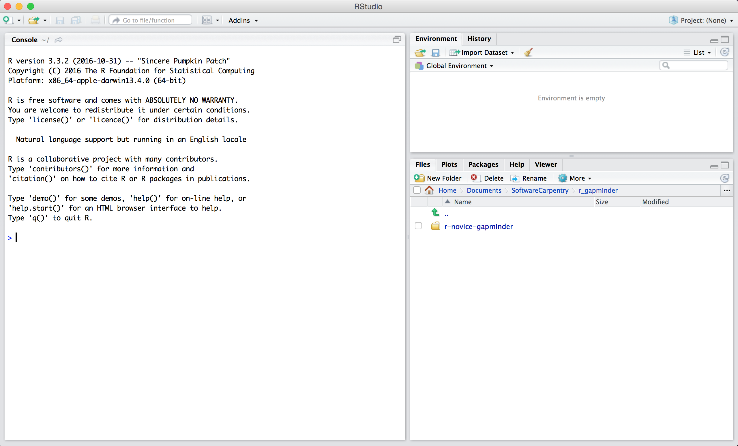
Once you open files, such as R scripts, an editor panel will also open in the top left.
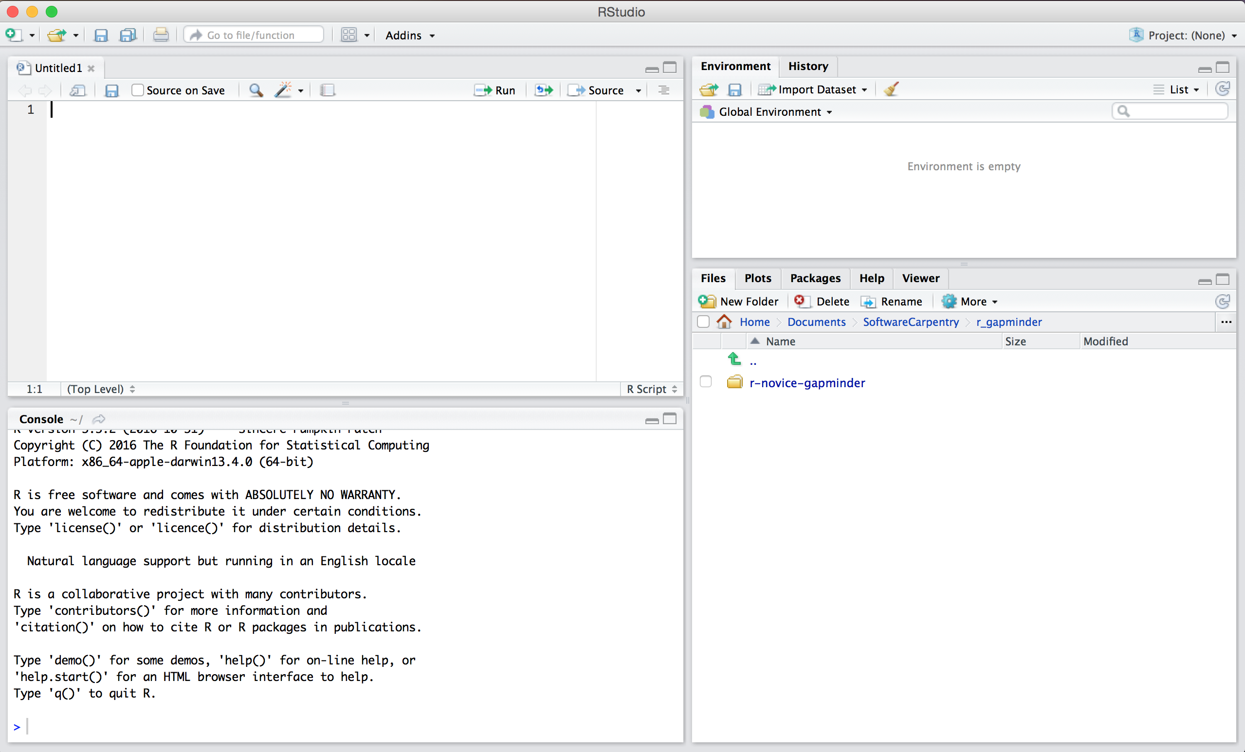
Tip: Do not save your working directory
When you exit R/RStudio, you probably get a prompt about saving your workspace image - don’t do this! In fact, it is recommended that you turn this feature off so you are not tempted: Go to Tools > Global Options and click “Never” in the dropdown next to “Save workspace to .RData on exit”
Creating a new project
One of the most powerful and useful aspects of RStudio is its project management functionality. We’ll be using this today to create a self-contained, reproducible project.
Challenge: Creating a self-contained project
We’re going to create a new project in RStudio:
- Click the “File” menu button, then “New Project”.
- Click “New Directory”.
- Click “Empty Project”.
- Type in the name of the directory to store your project, e.g. “EEOB546_R_lesson”.
- Make sure that the checkbox for “Create a git repository” is selected.
- Click the “Create Project” button.
Now when we start R in this project directory, or open this project with RStudio, all of our work on this project will be entirely self-contained in this directory.
Best practices for project organization
There are several general principles to adhere to that will make project management easier:
Treat data as read only
This is probably the most important goal of setting up a project. Data is typically time consuming and/or expensive to collect. Working with them interactively (e.g., in Excel) where they can be modified means you are never sure of where the data came from, or how it has been modified since collection. It is therefore a good idea to treat your data as “read-only”.
Data Cleaning
In many cases your data will be “dirty”: it will need significant preprocessing to get into a format R (or any other programming language) will find useful. This task is sometimes called “data munging”. It can be useful to store these scripts in a separate folder, and create a second “read-only” data folder to hold the “cleaned” data sets.
Treat generated output as disposable
Anything generated by your scripts should be treated as disposable: you should be able to regenerate it from your scripts.
Tip: Good Enough Practices for Scientific Computing
Good Enough Practices for Scientific Computing gives the following recommendations for project organization:
- Put each project in its own directory, which is named after the project.
- Put text documents associated with the project in the
docdirectory.- Put raw data and metadata in the
datadirectory, and files generated during cleanup and analysis in aresultsdirectory.- Put source for the project’s scripts and programs in the
srcdirectory, and programs brought in from elsewhere or compiled locally in thebindirectory.- Name all files to reflect their content or function.
Separate function definition and application
When your project is new and shiny, the script file usually contains many lines of directly executed code. As it matures, reusable chunks get pulled into their own functions. It’s a good idea to separate these into separate folders; one to store useful functions that you’ll reuse across analyses and projects, and one to store the analysis scripts.
Tip: avoiding duplication
You may find yourself using data or analysis scripts across several projects. Typically you want to avoid duplication to save space and avoid having to make updates to code in multiple places.
For this, you can use “symbolic links”, which are essentially shortcuts to files somewhere else on a filesystem. On Linux and OS X you can use the
ln -scommand, and on Windows you can either create a shortcut or use themklinkcommand from the windows terminal.
Challenge 1
Create a new readme file in the project directory you created and and some information about the project.
Version Control
We also set up our project to integrate with git, putting it under version control. RStudio has a nicer interface to git than shell, but is somewhat limited in what it can do, so you will find yourself occasionally needing to use the shell. Let’s go through and make an initial commit of our template files.
The workspace/history pane has a tab for “Git”. We can stage each file by checking the box: you will see a green “A” next to stage files and folders, and yellow question marks next to files or folders git doesn’t know about yet. RStudio also nicely shows you the difference between files from different commits.
Tip: versioning disposable output
Generally you do not want to version disposable output (or read-only data). You should modify the
.gitignorefile to tell git to ignore these files and directories.
Challenge 2
- Create a directory within your project called
graphs.- Modify the
.gitignorefile to containgraphs/so that this disposable output isn’t versioned.Add the newly created folders to version control using the git interface.
Solution to Challenge 2
This can be done with the command line:
$ mkdir graphs
$ echo "graphs/" >> .gitignore
Now we want to push the contents of this commit to GitHub, so it is also backed-up off site and available to collaborators.
Challenge 3
- In GitHub, create a New repository, called here
BCB546-R-Exercise. Don’t initialize it with a README file because we’ll be importing an existing repository…- Make sure you have a proper public key in your GitHub settings
- In RStudio, again click Tools -> Shell … . Enter:
$ echo "# BCB546-R-Exercise" >> README.md
$ git add README.md
$ git commit -m "first commit"
$ git remote add origin git@github.com/[path to your directory]
$ git push -u origin master
- Change README.md file to indicate the changes you made
- Commit and push it from the Git tab on the Environment/history panel of Rstudio.
Key Points
Use RStudio to create and manage projects with consistent layout.
Treat raw data as read-only.
Treat generated output as disposable.
Separate function definition and application.
Use version control.
R Language Basics
Overview
Teaching: 30 min
Exercises: 20 minQuestions
How to do simple calculations in R?
How to assign values to variables and call functions?
What are R’s vectors, vector data types, and vectorization?
How to install packages?
How can I get help in R?
What is an R Markdown file and how can I create one?
Objectives
To understand variables and how to assign to them
To be able to use mathematical and comparison operations
To be able to call functions
To be able to find and use packages
To be able to read R help files for functions and special operators.
To be able to seek help from your peers.
To be able to create and use R Markdown files

Introduction to R
R Operators
The simplest thing you could do with R is arithmetic:
1 + 100
[1] 101
Here we used to numbers and a + sign, which is called an operator.
An operator is a symbol that tells the compiler to perform specific mathematical
or logical manipulations.
Arithmetic operators
There are several arithmetic operators we can use and they should look familiar to you. If you use several of them (e.g., `5 + 2 *3), the order of operations is the same as you would have learned back in school. The list below is arranged from highest to lowest precedence:
Arithmetic operations
Operator Description ( ) Parentheses ^or**Exponents /Divide *Multiply -Subtract +Add Examples
3 + 5 * 2^5[1] 163Use parentheses to group operations in order to force the order of evaluation if it differs from the default, or to make clear what you intend.
((3 + 5) * 2)^5[1] 1048576Really small or large numbers get a scientific notation:
2/10000[1] 2e-04You can write numbers in scientific notation too:
5e3[1] 5000
Like bash, if you type in an incomplete command, R will wait for you to
complete it. Any time you hit return and the R session shows a + instead of a
>, it means it’s waiting for you to complete the command. If you want to cancel
a command you can simply hit “Esc” and RStudio will give you back the >
prompt.
Tip: Cancelling commands
If you’re using R from the commandline instead of from within RStudio, you need to use
Ctrl+Cinstead ofEscto cancel the command. This applies to Mac users as well!Cancelling a command isn’t only useful for killing incomplete commands: you can also use it to tell R to stop running code (for example if its taking much longer than you expect), or to get rid of the code you’re currently writing.
Relational Operators
R also has relational operators that allow us to do comparison:
R Relational Operators
Operator Description < Less than > Greater than <= Less than or equal to >= Greater than or equal to == Equal to != Not equal to Examples
1 == 1; # equality (note two equals signs, read as "is equal to")[1] TRUE1 != 1; # inequality (read as "is not equal to")[1] FALSE1 < 2; # less than[1] TRUE# etc
Comparing Numbers
Let’s compare
0.1 + 0.2and0.3. What do you think?0.1 + 0.2 == 0.3[1] FALSEWhat’s happened?
Computers may only represent decimal numbers with a certain degree of precision, so two numbers which look the same when printed out by R, may actually have different underlying representations and therefore be different by a small margin of error (called Machine numeric tolerance). So, unless you compare two integers, you should use theall.equalfunction:all.equal(0.1 + 0.2, 0.3)[1] TRUEFurther reading: http://floating-point-gui.de/
Other operators
There are several other types of operators:
- Logical Operators
- Assignment Operators
- Miscellaneous Operators
We will see some of them in the next section and talk more about them in latter lessons (but see here if you can’t wait). Before we do it, we need to introduce variables.
Variables and assignment
A variable provides us with named storage that our programs can manipulate.
We can store values in variables using the assignment operator <-:
x <- 1/40
Notice that assignment does not print a value. Instead, we stored it for later
in something called a variable. x now contains the value 0.025:
x
[1] 0.025
Look for the Environment tab in one of the panes of RStudio, and you will see
that x and its value have appeared. Our variable x can be used in place of a
number in any calculation that expects a number:
x^2
[1] 0.000625
Notice also that variables can be reassigned:
x <- 100
x used to contain the value 0.025 and and now it has the value 100.
Assignment values can contain the variable being assigned to:
x <- x + 1; #notice how RStudio updates its description of x on the top right tab
x
[1] 101
The right hand side of the assignment can be any valid R expression. The right hand side is fully evaluated before the assignment occurs.
Tip: A shortcut for assignment operator
IN RStudio, you can create the <- assignment operator in one keystroke using
Option -(that’s a dash) on OS X orAlt -on Windows/Linux.
It is also possible to use the = operator for assignment:
x = 1/40
But this is much less common among R users. So the recommendation is to use <-.
Naming variables
Variable names can contain letters, numbers, underscores and periods. They cannot start with a number nor contain spaces at all. Different people use different conventions for long variable names, these include
- periods.between.words
- underscores_between_words
- camelCaseToSeparateWords What you use is up to you, but be consistent.
Warning:
Notice, that R does not use a special symbol to distinguish between variable and simple text. Instead, the text is placed in double quotes “text”. If R complains that the object text does not exist, you probably forgot to use the quotes!
Reserved words
Reserved words in R programming are a set of words that have special meaning and cannot be used as an identifier (variable name, function name etc.). To view the list of reserved words you can type
help(reserved)or?reservedat the R command prompt.
Vectorization
One final thing to be aware of is that R is vectorized, meaning that variables and functions can have vectors as values. We can create vectors using several commands:
Vectorization
Command Description c(2, 4, 6)Join elements into a vector 1:5Create an integer sequence seq(2, 3, by=0.5)Create a sequence with a specific increment rep(1:2, times=3)Repeat a vector rep(1:2, each=3)Repeat elements of a vector Examples
1:5;[1] 1 2 3 4 52^(1:5);[1] 2 4 8 16 32x <- 1:5; 2^x;[1] 2 4 8 16 32
This is incredibly powerful; we will discuss this further in an upcoming lesson.
Notice that in the table above we see some functions that can be recognized by
parenthesis that follow one or more letters (e.g., seq(2, 3, by=0.5)). R has
many in-built functions which can be directly called in the program without
defining them first. We can also create and use our own functions referred as
user defined functions. You can see some additional examples of in-build
functions in this handy Cheat Sheet
Managing your environment
There are a few useful commands you can use to interact with the R session.
ls will list all of the variables and functions stored in the global environment
(your working R session):
ls() # to list files use list.files() function
[1] "args" "dest_md" "op" "src_rmd" "x"
Tip: hidden objects
Like in the shell,
lswill hide any variables or functions starting with a “.” by default. To list all objects, typels(all.names=TRUE)instead
Note here that we didn’t given any arguments to ls, but we still
needed to give the parentheses to tell R to call the function.
If we type ls by itself, R will print out the source code for that function!
ls
function (name, pos = -1L, envir = as.environment(pos), all.names = FALSE,
    pattern, sorted = TRUE)
{
    if (!missing(name)) {
        pos <- tryCatch(name, error = function(e) e)
        if (inherits(pos, "error")) {
            name <- substitute(name)
            if (!is.character(name))
                name <- deparse(name)
            warning(gettextf("%s converted to character string",
                sQuote(name)), domain = NA)
            pos <- name
        }
    }
    all.names <- .Internal(ls(envir, all.names, sorted))
    if (!missing(pattern)) {
        if ((ll <- length(grep("[", pattern, fixed = TRUE))) &&
            ll != length(grep("]", pattern, fixed = TRUE))) {
            if (pattern == "[") {
                pattern <- "\\["
                warning("replaced regular expression pattern '[' by  '\\\\['")
            }
            else if (length(grep("[^\\\\]\\[<-", pattern))) {
                pattern <- sub("\\[<-", "\\\\\\[<-", pattern)
                warning("replaced '[<-' by '\\\\[<-' in regular expression pattern")
            }
        }
        grep(pattern, all.names, value = TRUE)
    }
    else all.names
}
<bytecode: 0x7f9b3d394c38>
<environment: namespace:base>
You can use rm to delete objects you no longer need:
rm(x)
If you have lots of things in your environment and want to delete all of them,
you can pass the results of ls to the rm function:
rm(list = ls())
In this case we’ve combined the two. Like the order of operations, anything inside the innermost parentheses is evaluated first, and so on.
Tip: Warnings vs. Errors
Pay attention when R does something unexpected! Errors, like above, are thrown when R cannot proceed with a calculation. Warnings on the other hand usually mean that the function has run, but it probably hasn’t worked as expected.
In both cases, the message that R prints out usually give you clues how to fix a problem.
R Packages
It is possible to add functions to R by writing a package, or by obtaining a package written by someone else. There are over 7,000 packages available on CRAN (the comprehensive R archive network). R and RStudio have functionality for managing packages:
- You can see what packages are installed by typing
installed.packages() - You can install packages by typing
install.packages("packagename"), wherepackagenameis the package name, in quotes. - You can update installed packages by typing
update.packages() - You can remove a package with
remove.packages("packagename") - You can make a package available for use with
library(packagename)
Writing your own code
Good coding style is like using correct punctuation. You can manage without it, but it sure makes things easier to read. As with styles of punctuation, there are many possible variations. Google’s R style guide is a good place to start. The formatR package, by Yihui Xie, makes it easier to clean up poorly formatted code. Make sure to read the notes on the wiki before using it.
Looking for help
Reading Help files
R, and every package, provide help files for functions. To search for help use:
?function_name
help(function_name)
This will load up a help page in RStudio (or as plain text in R by itself).
Note that each help page is broken down into several sections, including Description, Usage, Arguments, Examples, etc.
Operators
To seek help on operators, use quotes:
?"+"
Getting help on packages
Many packages come with “vignettes”: tutorials and extended example documentation.
Without any arguments, vignette() will list all vignettes for all installed packages;
vignette(package="package-name") will list all available vignettes for
package-name, and vignette("vignette-name") will open the specified vignette.
If a package doesn’t have any vignettes, you can usually find help by typing
help("package-name").
When you kind of remember the function
If you’re not sure what package a function is in, or how it’s specifically spelled you can do a fuzzy search:
??function_name
When you have no idea where to begin
If you don’t know what function or package you need to use CRAN Task Views is a specially maintained list of packages grouped into fields. This can be a good starting point.
When your code doesn’t work: seeking help from your peers
If you’re having trouble using a function, 9 times out of 10,
the answers you are seeking have already been answered on
Stack Overflow. You can search using
the [r] tag.
If you can’t find the answer, there are two useful functions to help you ask a question from your peers:
?dput
Will dump the data you’re working with into a format so that it can be copy and pasted by anyone else into their R session.
sessionInfo()
R version 4.0.4 (2021-02-15)
Platform: x86_64-apple-darwin17.0 (64-bit)
Running under: macOS Catalina 10.15.7

Matrix products: default
BLAS:   /Library/Frameworks/R.framework/Versions/4.0/Resources/lib/libRblas.dylib
LAPACK: /Library/Frameworks/R.framework/Versions/4.0/Resources/lib/libRlapack.dylib

locale:
[1] en_US.UTF-8/en_US.UTF-8/en_US.UTF-8/C/en_US.UTF-8/en_US.UTF-8

attached base packages:
[1] stats     graphics  grDevices utils     datasets  methods   base

other attached packages:
[1] knitr_1.31

loaded via a namespace (and not attached):
[1] compiler_4.0.4 magrittr_2.0.1 tools_4.0.4    stringi_1.5.3  stringr_1.4.0
[6] xfun_0.22      evaluate_0.14
Will print out your current version of R, as well as any packages you have loaded.
Vocabulary
As with any language, it’s important to work on your R vocabulary. Here is a good place to start
Challenge 1
Which of the following are valid R variable names?
min_height
max.height
_age
.mass
MaxLength
min-length
2widths
celsius2kelvin
Solution to challenge 1
The following can be used as R variables:
min_height
max.height
MaxLength
celsius2kelvin
The following creates a hidden variable:
.massThe following will not be able to be used to create a variable
_age
min-length
2widths
Challenge 2
What will be the value of each variable after each statement in the following program?
mass <- 47.5
age <- 122
mass <- mass * 2.3
age <- age - 20
Solution to challenge 2
mass <- 47.5This will give a value of 47.5 for the variable mass
age <- 122This will give a value of 122 for the variable age
mass <- mass * 2.3This will multiply the existing value of 47.5 by 2.3 to give a new value of 109.25 to the variable mass.
age <- age - 20This will subtract 20 from the existing value of 122 to give a new value of 102 to the variable age.
Challenge 3
Clean up your working environment by deleting the mass and age variables.
Solution to challenge 3
We can use the
rmcommand to accomplish this taskrm(age, mass)
Challenge 4
Install packages in the
tidyversecollectionSolution to challenge 4
We can use the
install.packages()command to install the required packages.install.packages("tidyverse")
Challenge 5
Use help to find a function (and its associated parameters) that you could use to load data from a csv file in which columns are delimited with “\t” (tab) and the decimal point is a “.” (period). This check for decimal separator is important, especially if you are working with international colleagues, because different countries have different conventions for the decimal point (i.e. comma vs period). hint: use
??csvto lookup csv related functions.
```
Key Points
R has the usual arithmetic operators and mathematical functions.
Use
<-to assign values to variables.Use
ls()to list the variables in a program.Use
rm()to delete objects in a program.Use
install.packages()to install packages (libraries).Use
library(packagename)to make a package available for useUse
help()to get online help in R.
Data Structures
Overview
Teaching: 50 min
Exercises: 30 minQuestions
What are the basic data types in R?
How do I represent categorical information in R?
Objectives
To be aware of the different types of data.
To begin exploring data frames, and understand how it’s related to vectors, factors and lists.
To be able to ask questions from R about the type, class, and structure of an object.
Disclaimer: This lesson is based on a chapter from the Advanced R book.
Data structures
R’s base data structures can be organized by their dimensionality (1d, 2d, or nd) and whether they’re homogeneous (all contents must be of the same type) or heterogeneous (the contents can be of different types):
R’s base data structures
Homogeneous Heterogeneous 1d Atomic vector List 2d Matrix Data frame nd Array
Almost all other objects are built upon these foundations. Note that R has no 0-dimensional, or scalar types. Individual numbers or strings are vectors of length one.
Given an object, the best way to understand what data structures it’s composed
of is to use str(). str() is short for structure and it gives a compact,
human readable description of any R data structure.
Vectors
The basic data structure in R is the vector. Vectors come in two flavors: atomic vectors and lists. They have three common properties:
- Type,
typeof(), what it is. - Length,
length(), how many elements it contains. - Attributes,
attributes(), additional arbitrary metadata.
They differ in the types of their elements: all elements of an atomic vector must be the same type, whereas the elements of a list can have different types.
Atomic vectors
There are four common types of atomic vectors : logical, integer, double (often called numeric), and character.
Atomic vectors are usually created with c(), short for combine.
dbl_var <- c(1, 2.5, 4.5)
# With the L suffix, you get an integer rather than a double
int_var <- c(1L, 6L, 10L)
# Use TRUE and FALSE (or T and F) to create logical vectors
log_var <- c(TRUE, FALSE, T, F)
chr_var <- c("these are", "some strings")
Atomic vectors are always flat, even if you nest c()’s: Try c(1, c(2, c(3, 4)))
Missing values are specified with NA, which is a logical vector of length 1.
NA will always be coerced to the correct type if used inside c().
Coercion
All elements of an atomic vector must be the same type, so when you attempt to
combine different types they will be coerced to the most flexible type. The
coercion rules go: logical -> integer -> double -> complex -> character,
where -> can be read as are transformed into. You can try to force coercion
against this flow using the as. functions:
Challenge 1
Create the following vectors and predict their type:
a <- c("a", 1)
b <- c(TRUE, 1)
c <- c(1L, 10)
d <- c(a, b, c)
Solution to Challenge 1
typeof(a); typeof(b); typeof(c); typeof(d)[1] "character"[1] "double"[1] "double"[1] "character"
Coercion often happens automatically. Most mathematical functions (+, log,
abs, etc.) will coerce to a double or integer, and most logical operations
(&, |, any, etc) will coerce to a logical. You will usually get a warning
message if the coercion might lose information. If confusion is likely,
explicitly coerce with as.character(), as.double(), as.integer(), or
as.logical().
TIP
When a logical vector is coerced to an integer or double,
TRUEbecomes 1 andFALSEbecomes 0. This is very useful in conjunction withsum()andmean(), which will calculate the total number and proportion of “TRUE’s”, respectively.
Lists
Lists are one dimensional data structures that are different from atomic
vectors because their elements can be of any type, including lists. We construct
lists by using list() instead of c():
x <- c(1,2,3)
y <- list(1,2,3)
z <- list(1:3, "a", c(TRUE, FALSE, TRUE), c(2.3, 5.9))
RESULTS
str(x); str(y); str(z)num [1:3] 1 2 3List of 3 $ : num 1 $ : num 2 $ : num 3List of 4 $ : int [1:3] 1 2 3 $ : chr "a" $ : logi [1:3] TRUE FALSE TRUE $ : num [1:2] 2.3 5.9
Lists are sometimes called recursive vectors, because a list can contain other lists. This makes them fundamentally different from atomic vectors.
x <- list(list(list(list())))
str(x)
List of 1
 $ :List of 1
  ..$ :List of 1
  .. ..$ : list()
is.recursive(x)
[1] TRUE
c() will combine several lists into one. If given a combination of atomic
vectors and lists, c() will coerce the vectors to lists before combining them.
Example
Compare the results of
list()andc():x <- list(list(1, 2), c(3, 4)) y <- c(list(1, 2), c(3, 4)) str(x); str(y)List of 2 $ :List of 2 ..$ : num 1 ..$ : num 2 $ : num [1:2] 3 4List of 4 $ : num 1 $ : num 2 $ : num 3 $ : num 4
The typeof() a list is list. You can test for a list with is.list() and
coerce to a list with as.list(). You can turn a list into an atomic vector
with unlist(). If the elements of a list have different types, unlist() uses
the same coercion rules as c().
Discussion 1
What are the common types of atomic vector? How does a list differ from an atomic vector?
What will the commands
is.vector(list(1,2,3))is.numeric(c(1L,2L,3L))produce? How abouttypeof(as.numeric(c(1L,2L,3L)))?Test your knowledge of vector coercion rules by predicting the output of the following uses of
c():c(1, FALSE) c("a", 1) c(list(1), "a") c(TRUE, 1L)Why do you need to use
unlist()to convert a list to an atomic vector? Why doesn’tas.vector()work?Why is
1 == "1"true? Why is-1 < FALSEtrue? Why is"one" < 2false?Why is the default missing value,
NA, a logical vector? What’s special about logical vectors? (Hint: think aboutc(FALSE, NA)vs.c(FALSE, NA_character_).)
Attributes
All objects can have arbitrary additional attributes, used to store metadata
about the object. Attributes can be thought of as a named list (with unique names).
Attributes can be accessed individually with attr() or all at once (as a list)
with attributes().
The three most important attributes:
-
Names, a character vector giving each element a name, described in names.
-
Dimensions, used to turn vectors into matrices and arrays, described in matrices and arrays.
-
Class, used to implement the S3 object system.
Each of these attributes has a specific accessor function to get and set values:
names(x), dim(x), and class(x). To see
Names
You can name elements in a vector in three ways:
- When creating it:
x <- c(a = 1, b = 2, c = 3) - By modifying an existing vector in place:
x <- 1:3; names(x) <- c("a", "b", "c") - By creating a modified copy of a vector:
x <- 1:3; x <- setNames(x, c("a", "b", "c"))
You can see these names by just typing the vector’s name. You can access them
by using the names(x) function.
x <- 1:3;
x <- setNames(x, c("a", "b", "c"))
x
a b c
1 2 3
names(x)
[1] "a" "b" "c"
Names don’t have to be unique and not all elements of a vector need to have a name.
If some names are missing, names() will return an empty string for those elements.
If all names are missing, names() will return NULL.
You can create a new vector without names using unname(x), or remove names in
place with names(x) <- NULL.
Factors
One important use of attributes is to define factors. A factor is a vector that
can contain only predefined values, and is used to store categorical data.
Factors are built on top of integer vectors using two attributes: the class(),
“factor”, which makes them behave differently from regular integer vectors, and
the levels(), which defines the set of allowed values.
Examples
x <- c("a", "b", "b", "a")
x
[1] "a" "b" "b" "a"x <- factor(x) x[1] a b b a Levels: a bclass(x)[1] "factor"levels(x)[1] "a" "b"Factors are useful when you know the possible values a variable may take. Using a factor instead of a character vector makes it obvious when some groups contain no observations:
sex_char <- c("m", "m", "m")
sex_factor <- factor(sex_char, levels = c("m", "f"))

table(sex_char)
sex_char m 3table(sex_factor)sex_factor m f 3 0
Factors crip up all over R, and occasionally cause headaches for new R users.
Matrices and arrays
Adding a dim() attribute to an atomic vector allows it to behave like a
multi-dimensional array. An array with two dimensions is called matrix.
Matrices are used commonly as part of the mathematical
machinery of statistics. Arrays are much rarer, but worth being aware of.
Matrices and arrays are created with matrix() and array(),
or by using the assignment form of dim().
# Two scalar arguments to specify rows and columns
a <- matrix(1:6, ncol = 3, nrow = 2)
# One vector argument to describe all dimensions
b <- array(1:12, c(2, 3, 2))
# You can also modify an object in place by setting dim()
c <- 1:12
dim(c) <- c(3, 4)
c
     [,1] [,2] [,3] [,4]
[1,]    1    4    7   10
[2,]    2    5    8   11
[3,]    3    6    9   12
dim(c) <- c(4, 3)
c
     [,1] [,2] [,3]
[1,]    1    5    9
[2,]    2    6   10
[3,]    3    7   11
[4,]    4    8   12
dim(c) <- c(2, 3, 2)
c
, , 1

     [,1] [,2] [,3]
[1,]    1    3    5
[2,]    2    4    6

, , 2

     [,1] [,2] [,3]
[1,]    7    9   11
[2,]    8   10   12
You can test if an object is a matrix or array using is.matrix() and is.array(),
or by looking at the length of the dim(). as.matrix() and as.array() make
it easy to turn an existing vector into a matrix or array.
Discussion 2
What does
dim()return when applied to a vector?If
is.matrix(x)isTRUE, what willis.array(x)return?How would you describe the following three objects? What makes them different to
1:5?x1 <- array(1:5, c(1, 1, 5)) x2 <- array(1:5, c(1, 5, 1)) x3 <- array(1:5, c(5, 1, 1))
Data frames
A data frame is the most common way of storing data in R, and if used systematically makes data analysis easier. Under the hood, a data frame is a list of equal-length vectors. This makes it a 2-dimensional structure, so it shares properties of both the matrix and the list.
Useful Data Frame Functions
head()- shows first 6 rowstail()- shows last 6 rowsdim()- returns the dimensions of data frame (i.e. number of rows and number of columns)nrow()- number of rowsncol()- number of columnsstr()- structure of data frame - name, type and preview of data in each columnnames()- shows thenamesattribute for a data frame, which gives the column names.sapply(dataframe, class)- shows the class of each column in the data frame
Creation
You create a data frame using data.frame(), which takes named vectors as input:
df <- data.frame(x = 1:3, y = c("a", "b", "c"))
str(df)
'data.frame':	3 obs. of  2 variables:
 $ x: int  1 2 3
 $ y: chr  "a" "b" "c"
In R prior to v.4, data.frame()’s default behavior was to turn strings into
factors. Use stringAsFactors = FALSE to suppress this behavior!
df <- data.frame(
  x = 1:3,
  y = c("a", "b", "c"),
  stringsAsFactors = FALSE)
str(df)
'data.frame':	3 obs. of  2 variables:
 $ x: int  1 2 3
 $ y: chr  "a" "b" "c"
Testing and coercion
Because a data.frame is an S3 class, its type reflects the underlying vector
used to build it: the list. To check if an object is a data frame, use class()
or test explicitly with is.data.frame():
Examples
is.vector(df)[1] FALSEis.list(df)[1] TRUEis.data.frame(df)[1] TRUEtypeof(df)[1] "list"class(df)[1] "data.frame"
You can coerce an object to a data frame with as.data.frame():
- A vector will create a one-column data frame.
- A list will create one column for each element; it’s an error if they’re not all the same length.
- A matrix will create a data frame with the same number of columns and rows as the matrix.
Discussion 3
What attributes does a data frame possess?
What does
as.matrix()do when applied to a data frame with columns of different types?Can you have a data frame with 0 rows? What about 0 columns?
Key Points
Atomic vectors are usually created with
c(), short for combine;Lists are constructed by using
list();Data frames are created with
data.frame(), which takes named vectors as input;The basic data types in R are double, integer, complex, logical, and character;
All objects can have arbitrary additional attributes, used to store metadata about the object;
Adding a
dim()attribute to an atomic vector creates a multi-dimensional array;
Data Subsetting
Overview
Teaching: 30 min
Exercises: 10 minQuestions
How can I work with subsets of data in R?
Objectives
To be able to subset vectors, factors, lists, and dataframes
To be able to extract individual and multiple elements: by index, by name, using comparison operations
To be able to skip and remove elements from various data structures.
Disclaimer: This tutorial is partially based on an excellent book Advanced R.. Read chapter 4 to learn how to subset other data structures.
Subsetting
R has many powerful subset operators and mastering them will allow you to easily perform complex operations on any kind of dataset.
There are six different ways we can subset any kind of object, and three different subsetting operators for the different data structures.
Let’s start with the workhorse of R: atomic vectors.
Subsetting atomic vectors
By position
Code Meaning x[4]The fourth element x[-4]All but the forth x[2:4]Elements two to four x[-2:4]All except two to four x[c(1,5)Elements one and five
Important! Vector numbering in R starts at 1
In many programming languages (C and python, for example), the first element of a vector has an index of 0. In R, the first element is 1.
By name
Code Meaning x["b"]An element named “b”
Tip: Duplicated names
Although inexing by name is usually a much more reliable way to subset objects, notice, what will happen if we have several elements named “a”:
y <- c(5.4, 6.2, 7.1, 4.8, 7.5, 6.2)
names(y) <- c('a', 'b', 'c', 'a', 'e', 'a')
y[c("a", "c")]
a c 5.4 7.1We’ll solve this problem in the next section.
By position, value, or name using logical vectors
Code Meaning x[c(T,T,F)]Element at 1, 2, 4, 5, etc. postions x[all.equal(x, 6.2)]Element equal to 6.2 x[x < 3]All elements less than three x[names(x) == "a"All elements with name “a” x[names(x) %in% c("a", "c", "d")All elements with names “a”, “c”, or “d” x[!(names(x) %in% c("a","c","d"))]All elements with names other than “a”, “c”, “d”
Discussion 1
Predict and check the results of the following operations:
x <- c(5.4, 6.2, 7.1, 4.8, 7.5, 6.2)
names(x) <- c('a', 'b', 'c', 'd', 'e', 'f')
x[-(2:4)]
x[-2:4]
-x[2:4]
x[names(x) == "a"
Discuss with your neighbor subsetting using logical values. How does each of these commands work?
x[names(x) == "a"]x[which(names(x) == "a")produce the same results. How do these two commands differ from each other?
Tip: Getting help for operators
Remember you can search for help on operators by wrapping them in quotes:
help("%in%")or?"%in%".
Handling special values
At some point you will encounter functions in R which cannot handle missing, infinite, or undefined data.
There are a number of special functions you can use to filter out this data:
is.nawill return all positions in a vector, matrix, or data.frame containingNA.- likewise,
is.nan, andis.infinitewill do the same forNaNandInf.is.finitewill return all positions in a vector, matrix, or data.frame that do not containNA,NaNorInf.na.omitwill filter out all missing values from a vector
Subsetting lists: three functions: [, [[, and $.
1. Use [...] to return a subset of a list as a list.
If you want to subset a list, but not
extract an element, then you will likely use [...].
Examples
lst <- list(1:3, "a", c(TRUE, FALSE, TRUE), c(2.3, 5.9))
names(lst) <- c("A","B","C","D")
lst[1]
$A [1] 1 2 3str(lst[1])List of 1 $ A: int [1:3] 1 2 3
2. Use [[...]] to extract an individual element of a list.
You can’t extract more than one element at once nor use [[ ]] to skip elements:
Examples
lst <- list(1:3, "a", c(TRUE, FALSE, TRUE), c(2.3, 5.9))
names(lst) <- c("A","B","C","D")
lst[[1]]
[1] 1 2 3lst[["D"]][1] 2.3 5.9str(lst[[1]])int [1:3] 1 2 3lst[[1:3]]Error in lst[[1:3]]: recursive indexing failed at level 2lst[[-1]]Error in lst[[-1]]: invalid negative subscript in get1index <real>
3. Use $... to extract an element of a list by its name (you don’t need “” for the name):
Example
lst <- list(1:3, "a", c(TRUE, FALSE, TRUE), c(2.3, 5.9))
names(lst) <- c("A","B","C","D")
lst$D # The `$` function is a shorthand way for extracting elements by name
[1] 2.3 5.9
Discussion 2
What is the difference between these two commands? Did you get the results you expected?
lst <- list(1:3, "a", c(TRUE, FALSE, TRUE), c(2.3, 5.9))
names(lst) <- c("A","B","C","D")
# command 1:
lst[1][2]
# command 2:
lst[[1]][2]
Subsetting dataframes
Remember the data frames are lists underneath the hood, so similar rules apply. However they are also two dimensional objects!
Subset columns from a dataset using [...].
Remember the data frames are lists underneath the hood, so similar rules apply.
However, the resulting object will be a data frame:
## Example
df <- data.frame(
  x = 1:3,
  y = c("a", "b", "c"),
  z = c(TRUE,FALSE,TRUE),
  stringsAsFactors = FALSE)
str(df)
'data.frame': 3 obs. of 3 variables: $ x: int 1 2 3 $ y: chr "a" "b" "c" $ z: logi TRUE FALSE TRUEdf[1]x 1 1 2 2 3 3
Subset cells from a dataset using [...] with two numbers:
Example
The first argument corresponds to rows and the second to columns (either or both of them can be skipped!):
df[1:2,2:3]y z 1 a TRUE 2 b FALSEIf we subset a single row, the result will be a data frame (because the elements are mixed types):
df[3,]x y z 3 3 c TRUEBut for a single column the result will be a vector (this can be changed with the third argument,
drop = FALSE).df[,3][1] TRUE FALSE TRUE
Extract a single column using [[...]] or $... with the column name:
df$x
[1] 1 2 3
#or
df[["x"]]
[1] 1 2 3
Discussion 3
What is the difference between:
df[,2]
df[2]
df[[2]]
How about
  df[3,2] #and
  df[[2]][3]
Key Points
Access individual values by location using
[].Access slices of data using
[low:high].Access arbitrary sets of data using
[c(...)].Use
whichto select subsets of data based on value.
Data Transformation
Overview
Teaching: 60 min
Exercises: 30 minQuestions
How to use dplyr to transform data in R?
How do I select columns
How can I filter rows
How can I join two data frames?
Objectives
Be able to explore a dataframe
Be able to add, rename, and remove columns.
Be able to filter rows
Be able to append two data frames
Be able to join two data frames
Data transformation

Introduction
Every data analysis you conduct will likely involve manipulating dataframes at
some point. Quickly extracting, transforming, and summarizing information from
dataframes is an essential R skill. In this part we’ll use Hadley Wickham’s
dplyr package, which consolidates and simplifies many of the common operations
we perform on dataframes. In addition, much of dplyr key functionality is
written in C++ for speed.
Preliminaries
Inatall (if needed) and/or load two libraries, tidyverse and tidyr:
Dataset
Following chapter 8 of the Buffalo’s book, we will use the dataset Dataset_S1.txt from the paper “The Influence of Recombination on Human Genetic Diversity”. The dataset contains estimates of population genetics statistics such as nucleotide diversity (e.g., the columns Pi and Theta), recombination (column Recombination), and sequence divergence as estimated by percent identity between human and chimpanzee genomes (column Divergence). Other columns contain information about the sequencing depth (depth), and GC content (percent.GC) for 1kb windows in human chromosome 20. We’ll only work with a few columns in our examples; see the description of Dataset_S1.txt in the original paper for more details.
Download the dataset
We can download the Dataset_S1.txt file into a local folder of your choice using
the download.file function. Instead, we will read file directly from the
Internet with the read_csv function:
dvst <- read_csv("https://raw.githubusercontent.com/vsbuffalo/bds-files/master/chapter-08-r/Dataset_S1.txt")
── Column specification ─────────────────────────────────────────────────────────────────────────────────────────────────────────────────────────────────────────────────────────────────────────────────────
cols(
  start = col_double(),
  end = col_double(),
  `total SNPs` = col_double(),
  `total Bases` = col_double(),
  depth = col_double(),
  `unique SNPs` = col_double(),
  dhSNPs = col_double(),
  `reference Bases` = col_double(),
  Theta = col_double(),
  Pi = col_double(),
  Heterozygosity = col_double(),
  `%GC` = col_double(),
  Recombination = col_double(),
  Divergence = col_double(),
  Constraint = col_double(),
  SNPs = col_double()
)
Notice the parsing of columns in the file. Also notice that some of the columns names contain spaces and special characters. We’ll replace them soon to facilitate typing.
We can check the data structure creates with either the str(dvst) command or by
typing dvst:
dvst
# A tibble: 59,140 x 16
   start   end `total SNPs` `total Bases` depth `unique SNPs` dhSNPs
   <dbl> <dbl>        <dbl>         <dbl> <dbl>         <dbl>  <dbl>
 1 55001 56000            0          1894  3.41             0      0
 2 56001 57000            5          6683  6.68             2      2
 3 57001 58000            1          9063  9.06             1      0
 4 58001 59000            7         10256 10.3              3      2
 5 59001 60000            4          8057  8.06             4      0
 6 60001 61000            6          7051  7.05             2      1
 7 61001 62000            7          6950  6.95             2      1
 8 62001 63000            1          8834  8.83             1      0
 9 63001 64000            1          9629  9.63             1      0
10 64001 65000            3          7999  8                1      1
# … with 59,130 more rows, and 9 more variables: reference Bases <dbl>,
#   Theta <dbl>, Pi <dbl>, Heterozygosity <dbl>, %GC <dbl>,
#   Recombination <dbl>, Divergence <dbl>, Constraint <dbl>, SNPs <dbl>
It’s a tibble!. Notice that the tibble only shows the first few rows and all the columns that fit on one screen.
Run View(dvst), which will open the dataset in the RStudio viewer, to see the
whole dataframe.
Also notice that there are some additional variable types available:
| Abbreviation | Variable type |
|---|---|
int |
integers |
dbl |
doubles (real numbers) |
fctr |
factors (categorical) |
| Variables | not in the dataset |
chr |
character vectors (strings) |
dttm |
date-time |
lgl |
logical |
date |
dates |
dplyr basics
There are five key dplyr functions that allow you to solve the vast majority of data manipulation challenges:
Key
dplyrfunctions
Function Action filter()Pick observations by their values arrange()Reorder the rows select()Pick variables by their names mutate()Create new variables with functions of existing variables summarise()Collapse many values down to a single summary
None of these functions perform tasks you can’t accomplish with R’s base functions. But dplyr’s advantage is in the added consistency, speed, and versatility of its data manipulation interface. Get this cheatsheet to keep as a reminder of these and several additional functions.
group_by function
dplyr functions can be used in conjunction with group_by(), which changes
the scope of each function from operating on the entire dataset to operating on
it group-by-group.
Overall command structure
All dplyr functions work similarly:
-
The first argument is a data frame (actually, a
tibble). -
The subsequent arguments describe what to do with the data frame, using the variable names (without quotes).
-
The result is a new data frame.
Together these properties make it easy to chain together multiple simple steps to achieve a complex result.
These six functions provide the verbs for a language of data manipulation. Let’s dive in and see how these verbs work.
Use filter() to filter rows
Let’s say we used summary to get an idea about the total number of SNPs in
different windows:
summary(select(dvst,`total SNPs`)) # Here we also used `select` function. We'll talk about it soon.
   total SNPs
 Min.   : 0.000
 1st Qu.: 3.000
 Median : 7.000
 Mean   : 8.906
 3rd Qu.:12.000
 Max.   :93.000
The number varies considerably across all windows on chromosome 20 and the data are right-skewed: the third quartile is 12 SNPs, but the maximum is 93 SNPs. Often we want to investigate such outliers more closely.
We can use filter() to extract the rows of our dataframe based on their values.
The first argument is the name of the data frame. The second and subsequent
arguments are the expressions that filter the data frame.
filter(dvst,`total SNPs` >= 85)
# A tibble: 3 x 16
     start      end `total SNPs` `total Bases` depth `unique SNPs` dhSNPs
     <dbl>    <dbl>        <dbl>         <dbl> <dbl>         <dbl>  <dbl>
1  2621001  2622000           93         11337  11.3            13     10
2 13023001 13024000           88         11784  11.8            11      1
3 47356001 47357000           87         12505  12.5             9      7
# … with 9 more variables: reference Bases <dbl>, Theta <dbl>, Pi <dbl>,
#   Heterozygosity <dbl>, %GC <dbl>, Recombination <dbl>, Divergence <dbl>,
#   Constraint <dbl>, SNPs <dbl>
Questions:
- How many windows have >= 85 SNPs?
- What is a SNP?
We can build more elaborate queries by using multiple filters:
filter(dvst, Pi > 16, `%GC` > 80)
# A tibble: 3 x 16
     start      end `total SNPs` `total Bases` depth `unique SNPs` dhSNPs
     <dbl>    <dbl>        <dbl>         <dbl> <dbl>         <dbl>  <dbl>
1 63097001 63098000            5           947  2.39             2      1
2 63188001 63189000            2          1623  3.21             2      0
3 63189001 63190000            5          1395  1.89             3      2
# … with 9 more variables: reference Bases <dbl>, Theta <dbl>, Pi <dbl>,
#   Heterozygosity <dbl>, %GC <dbl>, Recombination <dbl>, Divergence <dbl>,
#   Constraint <dbl>, SNPs <dbl>
Note, dplyr functions never modify their inputs, so if you want to save the
result, you’ll need to use the assignment operator, <-:
new_df <- filter(dvst, Pi > 16, `%GC` > 80)
Tip
R either prints out the results, or saves them to a variable. If you want to do both, you can wrap the assignment in parentheses:
(new_df <- filter(dvst, Pi > 16, `%GC` > 80))
Comparisons
Use comparison operators to filter effectively:
>, >=, <, <=, != (not equal), and == (equal).
Remember, that == does not work well with real numbers! Use the dplyr near
function instead!
Logical operators
Multiple arguments to filter() are combined with “and”: every expression must
be true in order for a row to be included in the output. For other types of
combinations, you’ll need to use Boolean operators
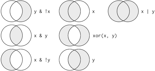
yourself: & is “and”, | is “or”, and ! is “not”. The figure below shows
the complete set of Boolean operations.
x %in% y operator
If you are looking for multiple values within a certain column, use the x %in% y
operator. This will select every row where x is one of the values in y:
filter(dvst, `total SNPs` %in% c(0,1,2))
# A tibble: 12,446 x 16
   start   end `total SNPs` `total Bases` depth `unique SNPs` dhSNPs
   <dbl> <dbl>        <dbl>         <dbl> <dbl>         <dbl>  <dbl>
 1 55001 56000            0          1894  3.41             0      0
 2 57001 58000            1          9063  9.06             1      0
 3 62001 63000            1          8834  8.83             1      0
 4 63001 64000            1          9629  9.63             1      0
 5 65001 66000            0          8376  8.38             0      0
 6 66001 67000            2          8431  8.43             2      0
 7 68001 69000            1          5381  5.38             1      0
 8 72001 73000            1          5276  5.28             1      0
 9 73001 74000            1          6648  6.65             1      0
10 80001 81000            1          6230  6.23             1      0
# … with 12,436 more rows, and 9 more variables: reference Bases <dbl>,
#   Theta <dbl>, Pi <dbl>, Heterozygosity <dbl>, %GC <dbl>,
#   Recombination <dbl>, Divergence <dbl>, Constraint <dbl>, SNPs <dbl>
Finally, whenever you start using complicated, multipart expressions in filter(),
consider making them explicit variables instead. That makes it much easier to
check your work. We’ll learn how to create new variables shortly.
Missing values
One important feature of R that can make comparison tricky are missing values, or
NAs (“not availables”).NArepresents an unknown value so missing values are “contagious”: almost any operation involving an unknown value will also be unknown.Examples:
NA > 5[1] NA10 == NA[1] NANA + 10[1] NANA / 2[1] NANA == NA[1] NA
filter() only includes rows where the condition is TRUE; it excludes both
FALSE and NA values. If you want
to preserve missing values, ask for them explicitly:
filter(dvst, is.na(Divergence))
Use mutate() to add new variables
It’s often useful to add new columns that are functions of existing columns.
That’s the job of mutate(). mutate() always adds new columns at the end of
your dataset. Remember that when you’re in RStudio, the easiest way to see all
the columns is with View().
Here we’ll add an additional column that indicates whether a window is in the centromere region (nucleotides 25,800,000 to 29,700,000, based on Giemsa banding; see README for details).
We’ll call it cent and make it logical (with TRUE/FALSE values):
mutate(dvst, cent = start >= 25800000 & end <= 29700000)
# A tibble: 59,140 x 17
   start   end `total SNPs` `total Bases` depth `unique SNPs` dhSNPs
   <dbl> <dbl>        <dbl>         <dbl> <dbl>         <dbl>  <dbl>
 1 55001 56000            0          1894  3.41             0      0
 2 56001 57000            5          6683  6.68             2      2
 3 57001 58000            1          9063  9.06             1      0
 4 58001 59000            7         10256 10.3              3      2
 5 59001 60000            4          8057  8.06             4      0
 6 60001 61000            6          7051  7.05             2      1
 7 61001 62000            7          6950  6.95             2      1
 8 62001 63000            1          8834  8.83             1      0
 9 63001 64000            1          9629  9.63             1      0
10 64001 65000            3          7999  8                1      1
# … with 59,130 more rows, and 10 more variables: reference Bases <dbl>,
#   Theta <dbl>, Pi <dbl>, Heterozygosity <dbl>, %GC <dbl>,
#   Recombination <dbl>, Divergence <dbl>, Constraint <dbl>, SNPs <dbl>,
#   cent <lgl>
dvst
# A tibble: 59,140 x 16
   start   end `total SNPs` `total Bases` depth `unique SNPs` dhSNPs
   <dbl> <dbl>        <dbl>         <dbl> <dbl>         <dbl>  <dbl>
 1 55001 56000            0          1894  3.41             0      0
 2 56001 57000            5          6683  6.68             2      2
 3 57001 58000            1          9063  9.06             1      0
 4 58001 59000            7         10256 10.3              3      2
 5 59001 60000            4          8057  8.06             4      0
 6 60001 61000            6          7051  7.05             2      1
 7 61001 62000            7          6950  6.95             2      1
 8 62001 63000            1          8834  8.83             1      0
 9 63001 64000            1          9629  9.63             1      0
10 64001 65000            3          7999  8                1      1
# … with 59,130 more rows, and 9 more variables: reference Bases <dbl>,
#   Theta <dbl>, Pi <dbl>, Heterozygosity <dbl>, %GC <dbl>,
#   Recombination <dbl>, Divergence <dbl>, Constraint <dbl>, SNPs <dbl>
Question:
Why don’t we see the column in the dataset?
In the dataset we are using, the diversity estimate Pi is measured per sampling window (1kb) and scaled up by 10x (see supplementary Text S1 for more details). It would be useful to have this scaled as per basepair nucleotide diversity (so as to make the scale more intuitive).
mutate(dvst, diversity = Pi / (10*1000)) # rescale, removing 10x and making per bp
# A tibble: 59,140 x 17
   start   end `total SNPs` `total Bases` depth `unique SNPs` dhSNPs
   <dbl> <dbl>        <dbl>         <dbl> <dbl>         <dbl>  <dbl>
 1 55001 56000            0          1894  3.41             0      0
 2 56001 57000            5          6683  6.68             2      2
 3 57001 58000            1          9063  9.06             1      0
 4 58001 59000            7         10256 10.3              3      2
 5 59001 60000            4          8057  8.06             4      0
 6 60001 61000            6          7051  7.05             2      1
 7 61001 62000            7          6950  6.95             2      1
 8 62001 63000            1          8834  8.83             1      0
 9 63001 64000            1          9629  9.63             1      0
10 64001 65000            3          7999  8                1      1
# … with 59,130 more rows, and 10 more variables: reference Bases <dbl>,
#   Theta <dbl>, Pi <dbl>, Heterozygosity <dbl>, %GC <dbl>,
#   Recombination <dbl>, Divergence <dbl>, Constraint <dbl>, SNPs <dbl>,
#   diversity <dbl>
Notice, that we can combine the two operations in a single command (and also save the result):
dvst <- mutate(dvst,
       diversity = Pi / (10*1000),
       cent = start >= 25800000 & end <= 29700000
)
If you only want to keep the new variables, use transmute():
transmute(dvst,
  diversity = Pi / (10*1000),
  cent = start >= 25800000 & end <= 29700000
)
# A tibble: 59,140 x 2
   diversity cent
       <dbl> <lgl>
 1  0        FALSE
 2  0.00104  FALSE
 3  0.000199 FALSE
 4  0.000956 FALSE
 5  0.000851 FALSE
 6  0.000912 FALSE
 7  0.000806 FALSE
 8  0.000206 FALSE
 9  0.000188 FALSE
10  0.000541 FALSE
# … with 59,130 more rows
Other creation functions
There are many functions for creating new variables that you can use with
mutate(). The key property is that the function must be vectorised: it must take a vector of values as input, return a vector with the same number of values as output. There’s no way to list every possible function that you might use, but here’s a selection of functions that are frequently useful:
Arithmetic operators:
+,-,*,/,^. These are all vectorised, using the so called “recycling rules”.Modular arithmetic:
%/%(integer division) and%%(remainder), wherex == y * (x %/% y) + (x %% y). Modular arithmetic is a handy tool because it allows you to break integers up into pieces.Logs:
log(),log2(),log10(). Logarithms are an incredibly useful transformation for dealing with data that ranges across multiple orders of magnitude. They also convert multiplicative relationships to additive.Offsets:
lead()andlag()allow you to refer to leading or lagging values. This allows you to compute running differences (e.g.x - lag(x)) or find when values change (x != lag(x)). They are most useful in conjunction withgroup_by(), which you’ll learn about shortly.Cumulative and rolling aggregates: R provides functions for running sums, products, mins and maxes:
cumsum(),cumprod(),cummin(),cummax(); and dplyr providescummean()for cumulative means.Logical comparisons,
<,<=,>,>=,!=, which you learned about earlier. If you’re doing a complex sequence of logical operations it’s often a good idea to store the interim values in new variables so you can check that each step is working as expected.Ranking:
min_rank()does the most usual type of ranking (e.g. 1st, 2nd, 2nd, 4th). The default gives smallest values the small ranks; usedesc(x)to give the largest values the smallest ranks. Ifmin_rank()doesn’t do what you need, look at the variantsrow_number(),dense_rank(),percent_rank(),cume_dist(),ntile(). See their help pages for more details.
Your turn!
- Find all sampling windows …
- with the lowest/highest GC content
- that have 0 total SNPs
- that are incomplete (<1000 bp)
- that have the highest divergence with the chimp
- that have less than 5% GC difference from the mean
- One useful dplyr filtering helper is
between().
- Can you figure out what does it do?
- Use it to simplify the code needed to answer the previous challenges.
- How many windows fall into the centromeric region?
Use arrange() to arrange rows
arrange() works similarly to filter() except that instead of selecting rows,
it changes their order. It takes a data frame and a set of column names (or more
complicated expressions) to order by. If you provide more than one column name,
each additional column will be used to break ties in the values of preceding
columns:
arrange(dvst, cent, `%GC`)
# A tibble: 59,140 x 18
      start      end `total SNPs` `total Bases` depth `unique SNPs` dhSNPs
      <dbl>    <dbl>        <dbl>         <dbl> <dbl>         <dbl>  <dbl>
 1 43448001 43449000            5           690  2.66             5      0
 2 14930001 14931000           19          3620  4.57             7      1
 3 37777001 37778000            3           615  1.12             3      0
 4 54885001 54886000            1          2298  3.69             1      0
 5 54888001 54889000           15          3823  3.87            11      1
 6 41823001 41824000           15          6950  6.95            10      4
 7 50530001 50531000           10          7293  7.29             2      2
 8 39612001 39613000           13          8254  8.25             5      3
 9 55012001 55013000            7          7028  7.03             7      0
10 22058001 22059000            4           281  1.2              4      0
# … with 59,130 more rows, and 11 more variables: reference Bases <dbl>,
#   Theta <dbl>, Pi <dbl>, Heterozygosity <dbl>, %GC <dbl>,
#   Recombination <dbl>, Divergence <dbl>, Constraint <dbl>, SNPs <dbl>,
#   diversity <dbl>, cent <lgl>
Use desc() to re-order by a column in descending order:
arrange(dvst, desc(cent), `%GC`)
# A tibble: 59,140 x 18
      start      end `total SNPs` `total Bases` depth `unique SNPs` dhSNPs
      <dbl>    <dbl>        <dbl>         <dbl> <dbl>         <dbl>  <dbl>
 1 25869001 25870000           10          7292  7.29             6      2
 2 29318001 29319000            2          6192  6.19             2      0
 3 29372001 29373000            5          7422  7.42             3      2
 4 26174001 26175000            1          7816  7.82             1      0
 5 26182001 26183000            2          6630  6.63             1      1
 6 25924001 25925000           30          7127  7.13            15      8
 7 26155001 26156000            0          9449  9.45             0      0
 8 25926001 25927000           21          8197  8.2             13      6
 9 29519001 29520000           15          8135  8.14            13      2
10 25901001 25902000            9          9126  9.13             5      2
# … with 59,130 more rows, and 11 more variables: reference Bases <dbl>,
#   Theta <dbl>, Pi <dbl>, Heterozygosity <dbl>, %GC <dbl>,
#   Recombination <dbl>, Divergence <dbl>, Constraint <dbl>, SNPs <dbl>,
#   diversity <dbl>, cent <lgl>
Note, that missing values are always sorted at the end!
Use select() to select columns and rename() to rename them
select() is not terribly useful with our data because they only have a few
variables, but you can still get the general idea:
# Select columns by name
select(dvst, start, end, Divergence)
# A tibble: 59,140 x 3
   start   end Divergence
   <dbl> <dbl>      <dbl>
 1 55001 56000    0.00301
 2 56001 57000    0.0180
 3 57001 58000    0.00701
 4 58001 59000    0.0120
 5 59001 60000    0.0240
 6 60001 61000    0.0160
 7 61001 62000    0.0120
 8 62001 63000    0.0150
 9 63001 64000    0.00901
10 64001 65000    0.00701
# … with 59,130 more rows
# Select all columns between depth and Pi (inclusive)
select(dvst, depth:Pi)
# A tibble: 59,140 x 6
   depth `unique SNPs` dhSNPs `reference Bases` Theta    Pi
   <dbl>         <dbl>  <dbl>             <dbl> <dbl> <dbl>
 1  3.41             0      0               556  0     0
 2  6.68             2      2              1000  8.01 10.4
 3  9.06             1      0              1000  3.51  1.99
 4 10.3              3      2              1000  9.93  9.56
 5  8.06             4      0              1000 12.9   8.51
 6  7.05             2      1              1000  7.82  9.12
 7  6.95             2      1              1000  8.60  8.06
 8  8.83             1      0              1000  4.01  2.06
 9  9.63             1      0              1000  3.37  1.88
10  8                1      1              1000  4.16  5.41
# … with 59,130 more rows
# Select all columns except those from start to percent.GC (inclusive)
select(dvst, -(start:`%GC`))
# A tibble: 59,140 x 6
   Recombination Divergence Constraint  SNPs diversity cent
           <dbl>      <dbl>      <dbl> <dbl>     <dbl> <lgl>
 1       0.00960    0.00301          0     0  0        FALSE
 2       0.00960    0.0180           0     0  0.00104  FALSE
 3       0.00960    0.00701          0     0  0.000199 FALSE
 4       0.00960    0.0120           0     0  0.000956 FALSE
 5       0.00960    0.0240           0     0  0.000851 FALSE
 6       0.00960    0.0160           0     0  0.000912 FALSE
 7       0.00960    0.0120           0     0  0.000806 FALSE
 8       0.00960    0.0150           0     0  0.000206 FALSE
 9       0.00960    0.00901         58     1  0.000188 FALSE
10       0.00958    0.00701          0     1  0.000541 FALSE
# … with 59,130 more rows
select() can also be used to rename variables, but it’s rarely useful because
it drops all of the variables not explicitly mentioned. Instead, use rename(),
which is a variant of select() that keeps all the variables that aren’t
explicitly mentioned:
dvst <- rename(dvst, total.SNPs = `total SNPs`,
       total.Bases = `total Bases`,
       unique.SNPs = `unique SNPs`,
       reference.Bases = `reference Bases`,
       percent.GC = `%GC`) #renaming all the columns that require ` `!
colnames(dvst)
 [1] "start"           "end"             "total.SNPs"      "total.Bases"
 [5] "depth"           "unique.SNPs"     "dhSNPs"          "reference.Bases"
 [9] "Theta"           "Pi"              "Heterozygosity"  "percent.GC"
[13] "Recombination"   "Divergence"      "Constraint"      "SNPs"
[17] "diversity"       "cent"
Another option is to use select() in conjunction with the everything() helper.
This is useful if you have a handful of variables you’d like to move to the start
of the data frame:
select(dvst, cent, everything())
# A tibble: 59,140 x 18
   cent  start   end total.SNPs total.Bases depth unique.SNPs dhSNPs
   <lgl> <dbl> <dbl>      <dbl>       <dbl> <dbl>       <dbl>  <dbl>
 1 FALSE 55001 56000          0        1894  3.41           0      0
 2 FALSE 56001 57000          5        6683  6.68           2      2
 3 FALSE 57001 58000          1        9063  9.06           1      0
 4 FALSE 58001 59000          7       10256 10.3            3      2
 5 FALSE 59001 60000          4        8057  8.06           4      0
 6 FALSE 60001 61000          6        7051  7.05           2      1
 7 FALSE 61001 62000          7        6950  6.95           2      1
 8 FALSE 62001 63000          1        8834  8.83           1      0
 9 FALSE 63001 64000          1        9629  9.63           1      0
10 FALSE 64001 65000          3        7999  8              1      1
# … with 59,130 more rows, and 10 more variables: reference.Bases <dbl>,
#   Theta <dbl>, Pi <dbl>, Heterozygosity <dbl>, percent.GC <dbl>,
#   Recombination <dbl>, Divergence <dbl>, Constraint <dbl>, SNPs <dbl>,
#   diversity <dbl>
Use summarise() to make summaries
The last key verb is summarise(). It collapses a data frame to a single row:
summarise(dvst, GC = mean(percent.GC, na.rm = TRUE), averageSNPs=mean(total.SNPs,
na.rm = TRUE), allSNPs=sum(total.SNPs))
# A tibble: 1 x 3
     GC averageSNPs allSNPs
  <dbl>       <dbl>   <dbl>
1  44.1        8.91  526693
summarise() is not terribly useful unless we pair it with group_by().
This changes the unit of analysis from the complete dataset to individual groups.
Then, when you use the dplyr verbs on a grouped data frame they’ll be
automatically applied “by group”. For example, if we applied exactly the same
code to a data frame grouped by position related to centromere:
by_cent <- group_by(dvst, cent)
summarise(by_cent, GC = mean(percent.GC, na.rm = TRUE), averageSNPs=mean(total.SNPs, na.rm = TRUE), allSNPs=sum(total.SNPs))
# A tibble: 2 x 4
  cent     GC averageSNPs allSNPs
  <lgl> <dbl>       <dbl>   <dbl>
1 FALSE  44.2        8.87  518743
2 TRUE   39.7       11.6     7950
Subsetting columns can be a useful way to summarize data across two different conditions. For example, we might be curious if the average depth in a window (the depth column) differs between very high GC content windows (greater than 80%) and all other windows:
by_GC <- group_by(dvst, percent.GC >= 80)
summarize(by_GC, depth=mean(depth))
# A tibble: 2 x 2
  `percent.GC >= 80` depth
  <lgl>              <dbl>
1 FALSE               8.18
2 TRUE                2.24
This is a fairly large difference, but it’s important to consider how many windows this includes.
Whenever you do any aggregation, it’s always a good idea to include either a count (n()),
or a count of non-missing values (sum(!is.na(x))). That way you can check that you’re not
drawing conclusions based on very small amounts of data:
summarize(by_GC, mean_depth=mean(depth), n_rows=n())
# A tibble: 2 x 3
  `percent.GC >= 80` mean_depth n_rows
  <lgl>                   <dbl>  <int>
1 FALSE                    8.18  59131
2 TRUE                     2.24      9
Your turn
As another example, consider looking at Pi by windows that fall in the centromere and those that do not. Does the centromer have higher nucleotide diversity than other regions in these data?
Solutions
Because cent is a logical vector, we can group by it directly:
by_cent <- group_by(dvst, cent)
summarize(by_cent, nt_diversity=mean(diversity), min=which.min(diversity), n_rows=n())
# A tibble: 2 x 4 cent nt_diversity min n_rows <lgl> <dbl> <int> <int> 1 FALSE 0.00123 1 58455 2 TRUE 0.00204 1 685Indeed, the centromere does appear to have higher nucleotide diversity than other regions in this data.
Useful summary functions
Just using means, counts, and sum can get you a long way, but R provides many other useful summary functions:
- Measures of location: we’ve used
mean(x), butmedian(x)is also useful.- Measures of spread:
sd(x),IQR(x),mad(x). The mean squared deviation, or standard deviation or sd for short, is the standard measure of spread. The interquartile rangeIQR()and median absolute deviationmad(x)are robust equivalents that may be more useful if you have outliers.- Measures of rank:
min(x),quantile(x, 0.25),max(x). Quantiles are a generalisation of the median. For example,quantile(x, 0.25)will find a value ofxthat is greater than 25% of the values, and less than the remaining 75%.- Measures of position:
first(x),nth(x, 2),last(x). These work similarly tox[1],x[2], andx[length(x)]but let you set a default value if that position does not exist (i.e. you’re trying to get the 3rd element from a group that only has two elements).- Counts: You’ve seen
n(), which takes no arguments, and returns the size of the current group. To count the number of non-missing values, usesum(!is.na(x)). To count the number of distinct (unique) values, usen_distinct(x).- Counts and proportions of logical values:
sum(x > 10),mean(y == 0). When used with numeric functions,TRUEis converted to 1 andFALSEto 0. This makessum()andmean()very useful:sum(x)gives the number ofTRUEs inx, andmean(x)gives the proportion.
Together group_by() and summarise() provide one of the tools that you’ll use
most commonly when working with dplyr: grouped summaries. But before we go any
further with this, we need to introduce a powerful new idea: the pipe.
Combining multiple operations with the pipe
It looks like we have been creating and naming several intermediate files in our analysis, even though we didn’t care about them. Naming things is hard, so this slows down our analysis.
There’s another way to tackle the same problem with the pipe, %>%:
dvst %>%
  rename(GC.percent = percent.GC) %>%
  group_by(GC.percent >= 80) %>%
  summarize(mean_depth=mean(depth, na.rm = TRUE), n_rows=n())
# A tibble: 2 x 3
  `GC.percent >= 80` mean_depth n_rows
  <lgl>                   <dbl>  <int>
1 FALSE                    8.18  59131
2 TRUE                     2.24      9
This focuses on the transformations, not what’s being transformed.
You can read it as a series of imperative statements: group, then summarise, then
filter,
where %>% stands for “then”.
Behind the scenes, x %>% f(y) turns into f(x, y), and x %>% f(y) %>% g(z)
turns into g(f(x, y), z) and so on.
Working with the pipe is one of the key criteria for belonging to the tidyverse.
The only exception is ggplot2: it was written before the pipe was discovered.
However, the next iteration of ggplot2, ggvis, is supposed to use the pipe.
RStudio Tip
A shortcut for
%>%is available in the newest RStudio releases under the keybinding CTRL + SHIFT + M (or CMD + SHIFT + M for OSX).
You can also review the set of available keybindings when within RStudio with the ALT + SHIFT + K.
Missing values
You may have wondered about the
na.rmargument we used above. What happens if we don’t set it? We may get a lot of missing values! That’s because aggregation functions obey the usual rule of missing values: if there’s any missing value in the input, the output will be a missing value. Fortunately, all aggregation functions have anna.rmargument which removes the missing values prior to computation: We could have also removed all the rows that have uknown position value prior to the analysis with thefilter(!is.na())command
Finally, one of the best features of dplyr is that all of these same methods also work with database connections. For example, you can manipulate a SQLite database with all of the same verbs we’ve used here.
Extra reading: tidy data
The collection tidyverse that we’ve been using is a universe of operation on tidy data. But what is tidy data?
Tidy data is a standard way of storing data where:
- Every column is variable.
- Every row is an observation.
- Every cell is a single value.
If you ensure that your data is tidy, you’ll spend less time fighting with the tools and more time working on your analysis. Learn more about tidy data in vignette(“tidy-data”).
tidyrpackage withintidyversehelps you create tidy datatidyr functions fall into five main categories:
- Pivotting which converts between long and wide forms. tidyr 1.0.0 introduces
pivot_longer()andpivot_wider(), replacing the olderspread()andgather()functions.- Rectangling, which turns deeply nested lists (as from JSON) into tidy tibbles.
- Nesting converts grouped data to a form where each group becomes a single row containing a nested data frame, and unnesting does the opposite.
- Splitting and combining character columns. Use
separate()andextract()to pull a single character column into multiple columns; useunite()to combine multiple columns into a single character column.- Handling missing values: Make implicit missing values explicit with
complete(); make explicit missing values implicit withdrop_na(); replace missing values with next/previous value withfill(), or a known value withreplace_na().
See https://tidyr.tidyverse.org/ for more info.Pivot Longer
pivot_longer()makes datasets longer by increasing the number of rows and decreasing the number of columns.
pivot_longer()is commonly needed to tidy wild-caught datasets as they often optimise for ease of data entry or ease of comparison rather than ease of analysis.Here is an example of an untidy dataset:
relig_income# A tibble: 18 x 11 religion `<$10k` `$10-20k` `$20-30k` `$30-40k` `$40-50k` `$50-75k` `$75-100k` <chr> <dbl> <dbl> <dbl> <dbl> <dbl> <dbl> <dbl> 1 Agnostic 27 34 60 81 76 137 122 2 Atheist 12 27 37 52 35 70 73 3 Buddhist 27 21 30 34 33 58 62 4 Catholic 418 617 732 670 638 1116 949 5 Don’t k… 15 14 15 11 10 35 21 6 Evangel… 575 869 1064 982 881 1486 949 7 Hindu 1 9 7 9 11 34 47 8 Histori… 228 244 236 238 197 223 131 9 Jehovah… 20 27 24 24 21 30 15 10 Jewish 19 19 25 25 30 95 69 11 Mainlin… 289 495 619 655 651 1107 939 12 Mormon 29 40 48 51 56 112 85 13 Muslim 6 7 9 10 9 23 16 14 Orthodox 13 17 23 32 32 47 38 15 Other C… 9 7 11 13 13 14 18 16 Other F… 20 33 40 46 49 63 46 17 Other W… 5 2 3 4 2 7 3 18 Unaffil… 217 299 374 365 341 528 407 # … with 3 more variables: $100-150k <dbl>, >150k <dbl>, # Don't know/refused <dbl>This dataset contains three variables:
religion, stored in the rows,incomespread across the column names, andcountstored in the cell values.To tidy it we use
pivot_longer():relig_income %>% pivot_longer(-religion, names_to = "income", values_to = "count")# A tibble: 180 x 3 religion income count <chr> <chr> <dbl> 1 Agnostic <$10k 27 2 Agnostic $10-20k 34 3 Agnostic $20-30k 60 4 Agnostic $30-40k 81 5 Agnostic $40-50k 76 6 Agnostic $50-75k 137 7 Agnostic $75-100k 122 8 Agnostic $100-150k 109 9 Agnostic >150k 84 10 Agnostic Don't know/refused 96 # … with 170 more rows
- The first argument is the dataset to reshape, relig_income.
- The second argument describes which columns need to be reshaped. In this case, it’s every column apart from religion.
- The names_to gives the name of the variable that will be created from the data stored in the column names, i.e. income.
- The values_to gives the name of the variable that will be created from the data stored in the cell value, i.e. count.
See https://tidyr.tidyverse.org/articles/pivot.html for more info.
Key Points
Read in a csv file using
read_csv()View a dataframe with
ViewUse
filter()to pick observations by their valuesUse
arrange()to order the rowsUse
select()to pick variables by their namesUse
mutate()to create new variables with functions of existing variablesUse
summarize()to collapse many values down to a single summary
Visualizing Data
Overview
Teaching: 60 min
Exercises: 30 minQuestions
How can I explore my data by visualization in R?
Objectives
To be able to use ggplot2 to visuzlize your data
To understand the basic grammar of graphics, including the aesthetics and geometry layers, adding statistics, transforming scales, and coloring or panelling by groups.
Data visualization
Introduction
“The simple graph has brought more information to the data analyst’s mind than any other device.” — John Tukey
In this lesson we will learn how to visualize your data using ggplot2. R has several systems for making graphs, but ggplot2 is probably the most versatile. ggplot2 implements the grammar of graphics, a coherent system for describing and building graphs. With ggplot2, you can do more faster by learning one system and applying it in many places.
The lesson is based on Chapter 8 of the Bioinformatics Data Skills book by Vince Buffalo and Chapter 2 of the R for Data Science book by Garrett Grolemund and Hadley Wickham.
Additional Resources
- Download the ggplot2 cheatsheet and keep it handy while you are working with the package.
- See the official ggplot2 page for additional resources (including free books).
Prerequisites
ggplot2 is one of the core members of the tidyverse. So begin by loading it with:
library(tidyverse)
# I assume it is installed by now, but see previous episodes if you get an error message!
Dataset #1
We will again use the dataset Dataset_S1.txt from the paper
“The Influence of Recombination on Human Genetic Diversity”.
See the previous lesson for its description.
Let’s read it as a tibble and modify as we did before:
dvst <- read_csv("https://raw.githubusercontent.com/vsbuffalo/bds-files/master/chapter-08-r/Dataset_S1.txt") %>%
  mutate(diversity = Pi / (10*1000), cent = (start >= 25800000 & end <= 29700000)) %>%
  rename(percent.GC = `%GC`, total.SNPs = `total SNPs`, total.Bases = `total Bases`, reference.Bases = `reference Bases`)
Exploring Data Visually with ggplot2 I: Scatterplots and Densities
We’ll start by using ggplot2 to create a scatterplot of nucleotide diversity along the chromosome. But because our data is window-based, we’ll first add a column called position that’s the midpoint for each window:
dvst <- mutate(dvst, position = (end + start) / 2)
Now we make a ggplot:
ggplot(data = dvst) + geom_point(mapping=aes(x=position, y=diversity))
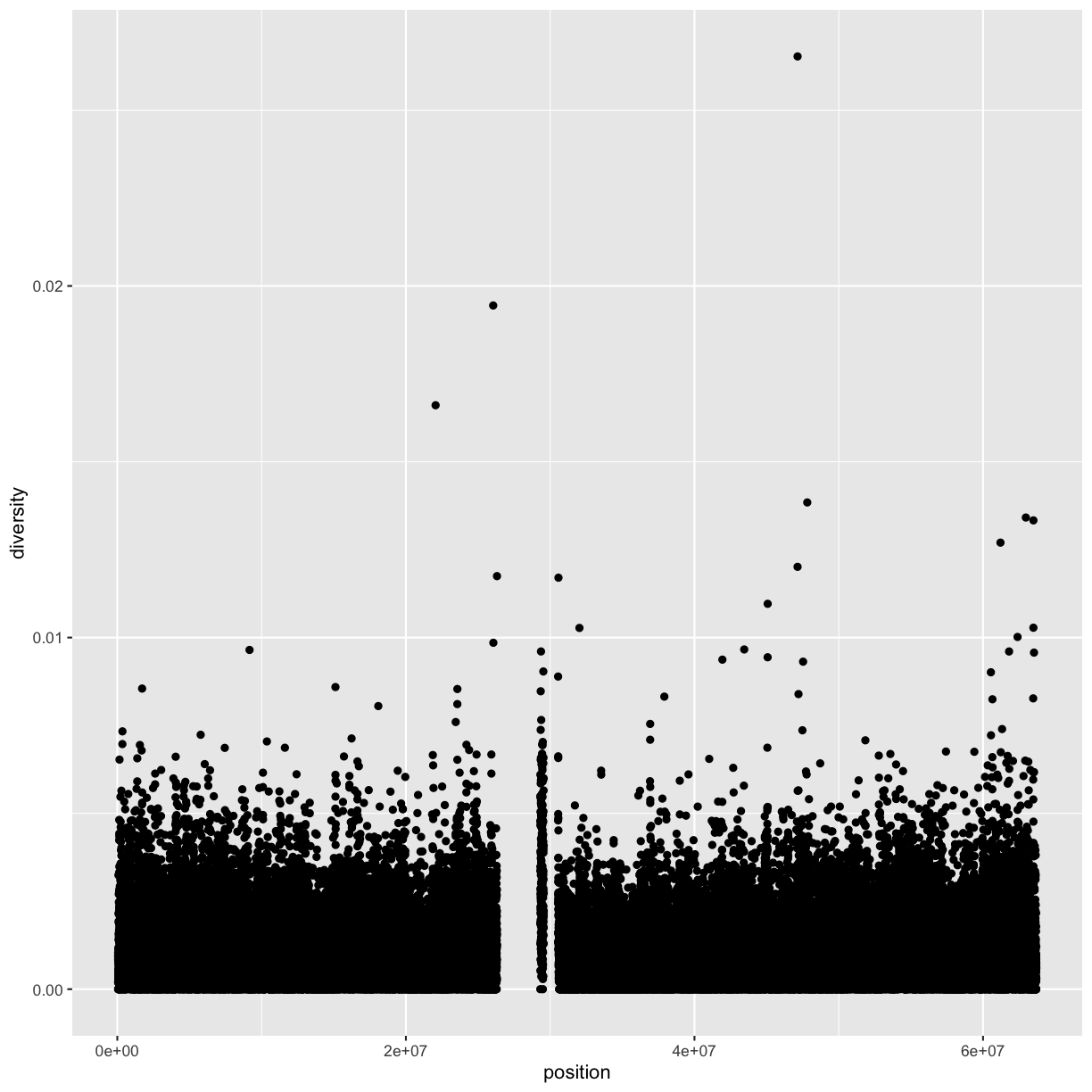
Note
With ggplot2, you begin a plot with the function
ggplot().ggplot()creates a coordinate system that you can add layers to. The first argument ofggplot()is the dataset to use in the graph. Soggplot(data = dvrs)creates an empty graph.You complete your graph by adding one or more layers to
ggplot().geom_point()is a type of geometric object (or geom in ggplot2 lingo) that creates a scatterplot. Note, that to add a layer, we use the same+operator that we use for addition in R.Each geom function in ggplot2 takes a
mappingargument. This defines how variables in your dataset are mapped to visual properties. Themappingargument is always paired withaes(), and thexandyarguments ofaes()specify which variables to map to the x and y axes. ggplot2 looks for the mapped variable in thedataargument, in this case,dvst.
A graphing template
We can use the code above to make a reusable template for making graphs with ggplot2. To make a graph, replace the bracketed sections in the code below with a dataset, a geom function, or a collection of mappings.
ggplot(data = <DATA>) +
  <GEOM_FUNCTION>(mapping = aes(<MAPPINGS>))
ggplot2 has many geoms (e.g., geom_line(), geom_bar(), etc). We’ll talk about them later.
Aesthetic mappings
“The greatest value of a picture is when it forces us to notice what we never expected to see.” — John Tukey
Notice the missing diversity estimates in the middle of this plot. What’s going on in this region? We can explore this question easily in ggplot by mapping a possible confounder or explanatory variable to another aesthetic. In this case, let’s map the color aesthetic of our point geometric objects to the column cent, which indicates whether the window falls in the centromeric region of this chromosome
ggplot(data = dvst) + geom_point(mapping = aes(x=position, y=diversity, color=cent))
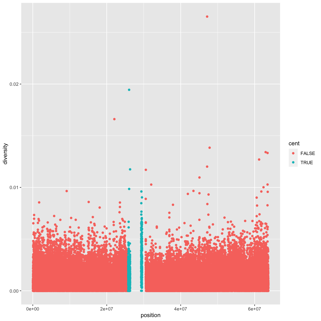
Note
Geometric objects have many aesthetic attributes (e.g., color, shape, size, etc.). You can map any of the geometric objects’ aesthetics to columns in your dataframe. The syntax highlights a useful insight about
xandy: the x and y locations of a point are themselves aesthetics, visual properties that you can map to variables to display information about the data. Once you map an aesthetic, ggplot2 takes care of the rest. It selects a reasonable scale to use with the aesthetic, and it constructs a legend that explains the mapping between levels and values. For x and y aesthetics, ggplot2 does not create a legend, but it creates an axis line with tick marks and a label. The axis line acts as a legend: it explains the mapping between locations and values.
You can also set the aesthetic properties of your geom manually. For example, we can make all of the points in our plot blue:
ggplot(data = dvst) +
  geom_point(mapping = aes(x = position, y = diversity), color = "blue")
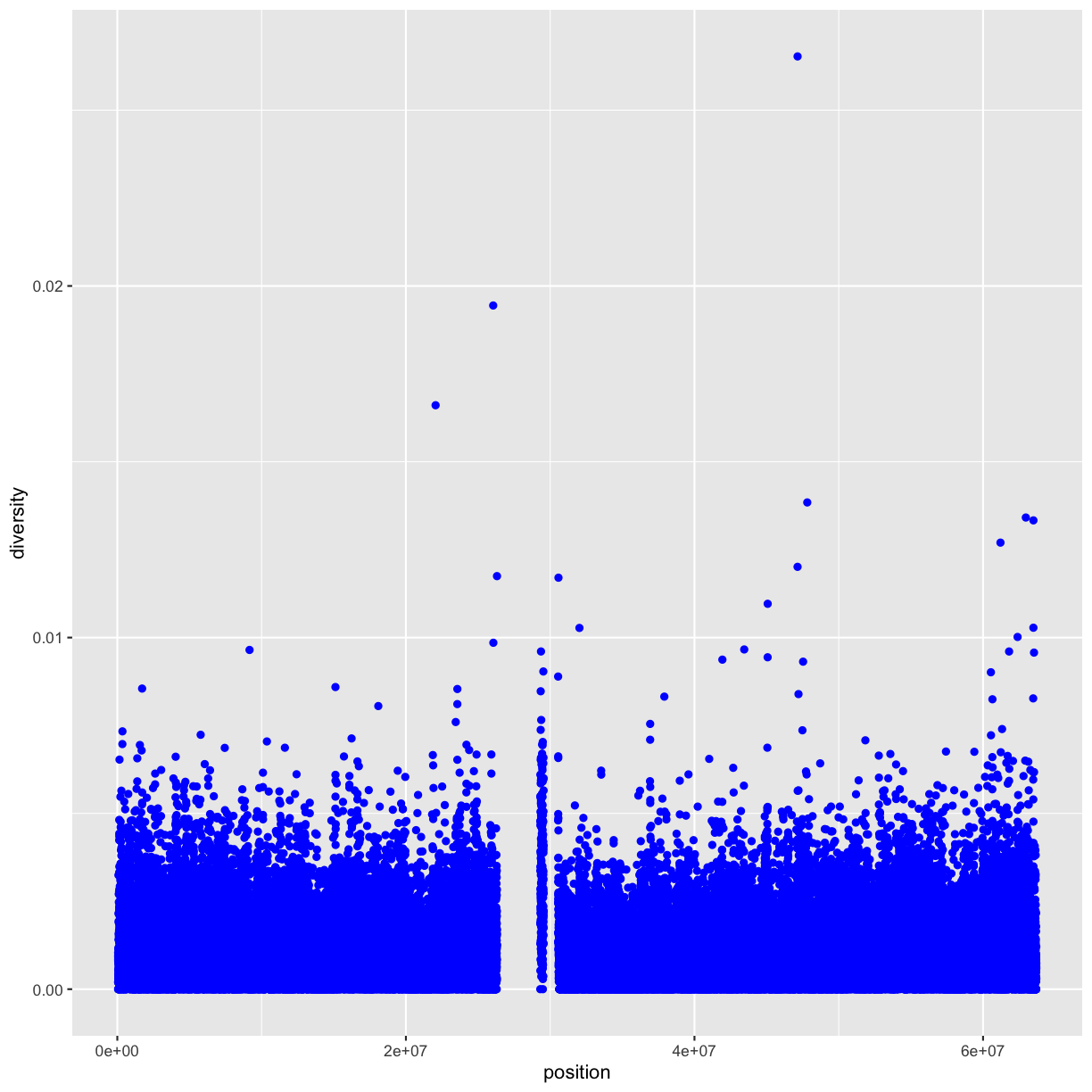
Here, the color doesn’t convey information about a variable, but only changes the
appearance of the plot. To set an aesthetic manually, set the aesthetic by name
as an argument of your geom function; i.e. it goes outside of aes(). You’ll
need to pick a value that makes sense for that aesthetic:
- The name of a color as a character string.
- The size of a point in mm.
- The shape of a point as a number, as shown below.

Finally, note, that aesthetic mappings can also be specified in the call to ggplot(); different geoms will then use this mapping:
ggplot(data = dvst, mapping = (aes(x=position, y=diversity))) + geom_point()
Discussion
What’s gone wrong with this code? Why are the points not blue?
ggplot(data = dvst) + geom_point(mapping = aes(x = position, y = diversity, color = "blue"))
Map a continuous variable to
color,size, andshape. How do these aesthetics behave differently for categorical vs. continuous variables?What happens if you map the same variable to multiple aesthetics?
What does the
strokeaesthetic do? What shapes does it work with? (Hint: use?geom_point)What happens if you map an aesthetic to something other than a variable name, like
aes(colour = percent.GC < 50)?
Common problems
As you start to run R code, you’re likely to run into problems. Don’t worry — it happens to everyone! Here a a few common problems (and solutions):
- Make sure that every
(is matched with a)and every"is paired with another".- Sometimes you’ll run the code and nothing happens. Check the left-hand of your console: if it’s a
+, it means that R doesn’t think you’ve typed a complete expression and it’s waiting for you to finish it. In this case, it’s usually easy to start from scratch again by pressing ESCAPE to abort processing the current command.- One common problem when creating ggplot2 graphics is to put the
+in the wrong place: it has to come at the end of the line, not the start. In other words, make sure you haven’t accidentally written code like this:ggplot(data = dvst) \+ geom_point(mapping = aes(x = position, y = diversity))
Overplotting
One problem with scatterplots (and our plot in particular) is overplotting (some data points obscure the information of other data points). We can’t get a sense of the distribution of diversity from this figure because everything is saturated from about 0.05 and below. One way to alleviate overplotting is to make points somewhat transparent (the transparency level is known as the alpha):
ggplot(data = dvst) + geom_point(mapping = aes(x=position, y=diversity), alpha=0.01)
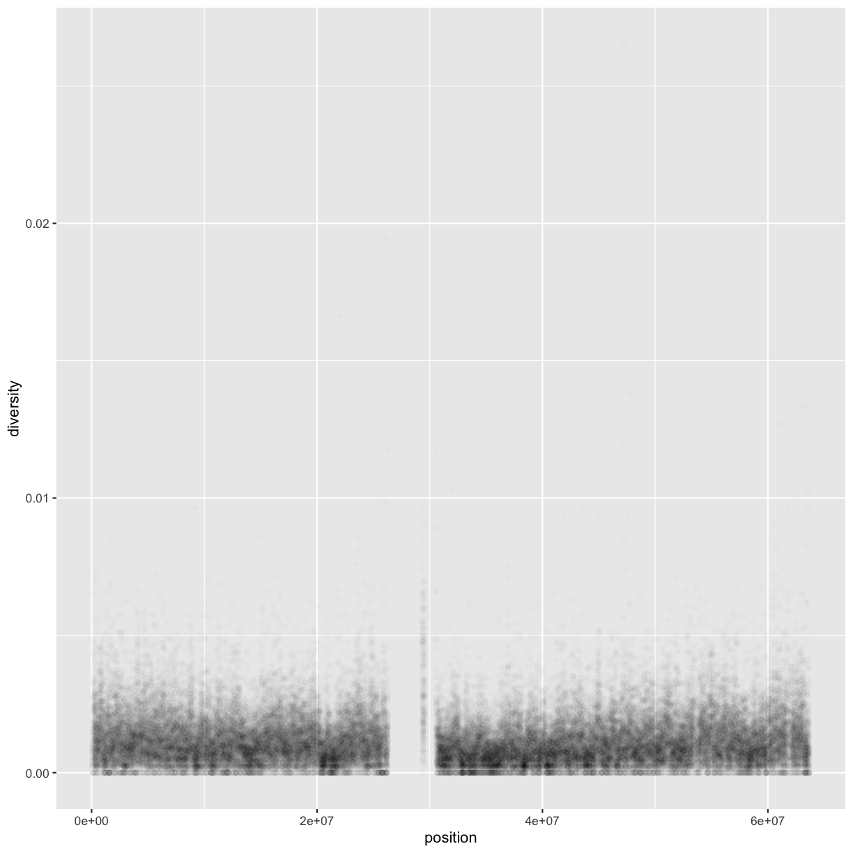 Note that we set alpha=0.01 outside of the aesthetic mapping function aes() as we did with the color in
the previous example. This is because we’re not mapping the alpha aesthetic to a column of data in our dataframe,
but rather givi0ng it a fixed value for all data points.
Density
Let’s now look at the density of diversity across all positions. We’ll use a different geometric object,
geom_density(), which is slightly different than geom_point() in that it takes the data and calculates
a density from it for us:
ggplot(data = dvst) + geom_density(mapping = aes(x=diversity), fill="blue")
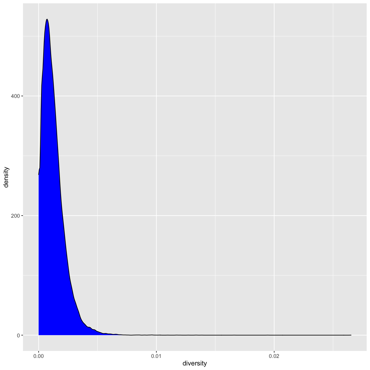
We can also map the color aesthetic of geom_density() to a discrete-valued column in our dataframe,
just as we did with geom_point(). geom_density() will create separate density plots, grouping data
by the column mapped to the color aesthetic and using colors to indicate the different densities.
To see both overlapping densities, we use alpha to set the transparency to 0.4:
ggplot(data = dvst) + geom_density(mapping = aes(x=diversity, fill=cent), alpha=0.4)
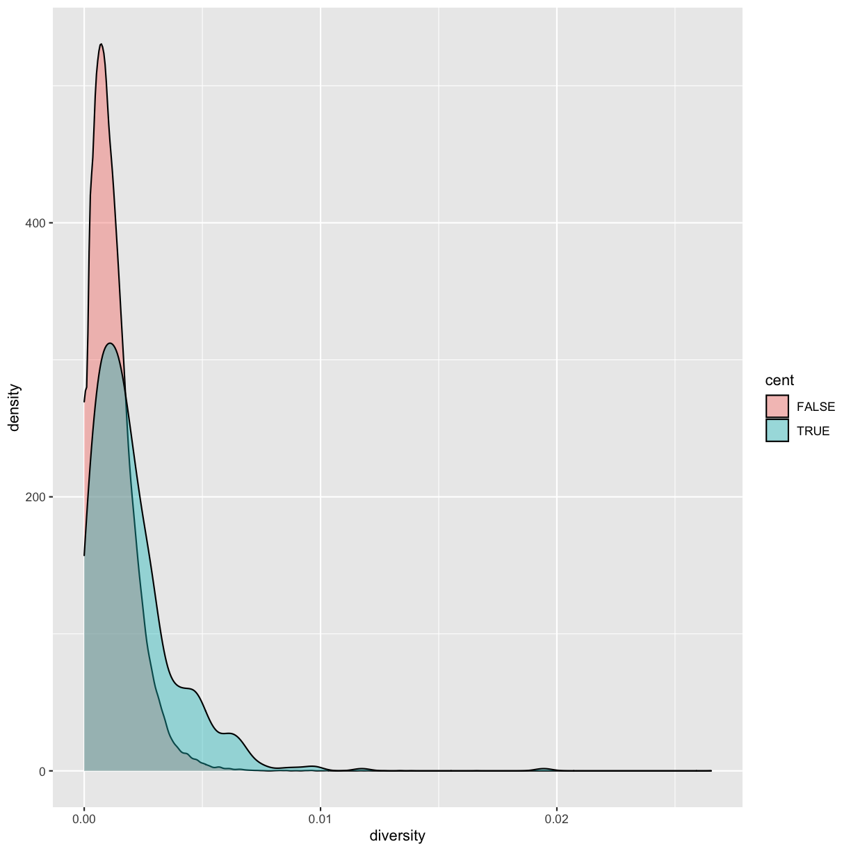
Immediately we’re able to see a trend that wasn’t clear by using a scatterplot: diversity is skewed to more extreme values in centromeric regions. Again (because this point is worth repeating), mapping columns to additional aesthetic attributes can reveal patterns and information in the data that may not be apparent in simple plots.
Exploring Data Visually with ggplot2 II: Smoothing
Let’s look at the Dataset_S1.txt data using another useful ggplot2 feature: smoothing. In particular, we’ll investigate potential confounders in genomic data. There are several potential factor that influence our estimates: sequencing read depth; GC content; mapability, or whether a region is capable of having reads correctly align to it; batch effects; etc. Often with large and high-dimension datasets, visualization is the easiest and best way to spot these potential issues.
Earlier, we used transparency to give us a sense of the most dense regions. Another
strategy is to use ggplot2’s geom_smooth() to add a smoothing line to plots and look
for an unexpected trend. Let’s use a scatterplot and smoothing curve to look at the
relationship between the sequencing depth (the depth column) and the total number of
SNPs in a window (the total.SNPs column):
ggplot(data = dvst, mapping = aes(x=depth, y=total.SNPs)) + geom_point(alpha=0.1) + geom_smooth()
`geom_smooth()` using method = 'gam' and formula 'y ~ s(x, bs = "cs")'
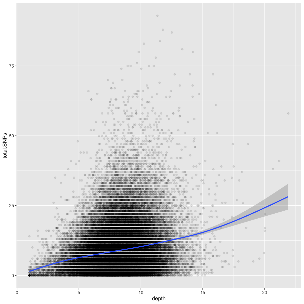
Notice that because both geom_point() and geom_smooth() use the same x and y mapping, we can specify
the aesthetic in ggplot() function.
Discussion
- What does this graph tells us about the relationship between depth of sequencing and SNPs?
- Why did we put the aesthetic mappings in the call to
ggplot()?- Try to add the
geom_smooth()function to the diversity graphs shown above. Is it more or less informative than usinggeom_density()? Why?
Challenge 1
Explore the effect GC content has on depth of sequencing in the dataset.
Solution to challenge 1
ggplot(data = dvst, mapping = aes(x=percent.GC, y=depth)) + geom_point() + geom_smooth()`geom_smooth()` using method = 'gam' and formula 'y ~ s(x, bs = "cs")'
Challenge 2
While ggplot2 chooses smart labels based on your column names, you might want to change this down the road. ggplot2 makes specifying labels easy: simply use the
xlab(),ylab(), andggtitle()functions to specify the x-axis label, y-axis label, and plot title. Change x- and y-axis labels when plotting the diversity data with x label “chromosome position (basepairs)” and y label “nucleotide diversity”.Solution to challenge 2
ggplot(dvst) + geom_point(aes(x=position, y=diversity)) + xlab("chromosome position (basepairs)") + ylab("nucleotide diversity")
Binning Data with cut() and Bar Plots with ggplot2
Next, let’s take a look at a bar chart. Bar charts seem simple, but they reveal something subtle about plots.
Consider a basic bar chart, as drawn with geom_bar(). As you can see, there are ~60000 windows in the dataset,
most of them outside the centromeric region.
ggplot(data = dvst) +
  geom_bar(mapping = aes(x = cent))

On the x-axis, the chart displays cent, a variable from dvst. On the y-axis, it displays count,
but count is not a variable in dvst! Where does count come from? Many graphs, like scatterplots,
plot the raw values of your dataset. Other graphs, like bar charts, calculate new values to plot:
-
bar charts, histograms, and frequency polygons bin your data and then plot bin counts, the number of points that fall in each bin.
-
smoothers fit a model to your data and then plot predictions from the model.
-
boxplots compute a robust summary of the distribution and then display a specially formatted box.
The algorithm used to calculate new values for a graph is called a stat, short for statistical transformation.
For example, geom_bar() uses stat_count() that simply counts the number of observations.
Extra reading: more about stats
You can learn which stat a geom uses by inspecting the default value for the
statargument. For example,?geom_barshows that the default value forstatis “count”, which means thatgeom_bar()usesstat_count().stat_count()is documented on the same page asgeom_bar(), and if you scroll down you can find a section called “Computed variables”. That describes how it computes two new variables:countandprop.You can generally use geoms and stats interchangeably. For example, you can recreate the previous plot using
stat_count()instead ofgeom_bar():ggplot(data = dvst) + stat_count(mapping = aes(x = cent))
This works because every geom has a default stat; and every stat has a default geom. This means that you can typically use geoms without worrying about the underlying statistical transformation. There are three reasons you might need to use a stat explicitly:
You might want to override the default stat. For example, the height of the bar may be already present in the data as another variable, in which case you will use
stat = "identity"You might want to override the default mapping from transformed variables to aesthetics. For example, you might want to display a bar chart of proportion, rather than count:
ggplot(data = dvst) +
  geom_bar(mapping = aes(x = cent, y = ..prop.., group = 1))
You might want to draw greater attention to the statistical transformation in your code. For example, you might use
stat_summary(), which summarises the y values for each unique x value, to draw attention to the summary that you’re computing:ggplot(data = dvst) + stat_summary( mapping = aes(x = cent, y = percent.GC), fun.ymin = min, fun.ymax = max, fun.y = median )Warning: `fun.y` is deprecated. Use `fun` instead.Warning: `fun.ymin` is deprecated. Use `fun.min` instead.Warning: `fun.ymax` is deprecated. Use `fun.max` instead.
ggplot2 provides over 20 stats for you to use. Each stat is a function, so you can get help in the usual way, e.g.
?stat_bin. To see a complete list of stats, check the ggplot2 cheatsheet.
Grouping data
So far we used cent, the only discrete variable in our dataset. Let’s create another one by
splitting the percent.GC into 5 categories:
dvst <- dvst %>%
  mutate(GC.binned = cut(percent.GC, 5));
select(dvst, GC.binned)
# A tibble: 59,140 x 1
   GC.binned
   <fct>
 1 (51.6,68.5]
 2 (34.7,51.6]
 3 (34.7,51.6]
 4 (34.7,51.6]
 5 (34.7,51.6]
 6 (34.7,51.6]
 7 (34.7,51.6]
 8 (34.7,51.6]
 9 (34.7,51.6]
10 (17.7,34.7]
# … with 59,130 more rows
ggplot(data = dvst) + geom_bar(mapping = aes(x=GC.binned))
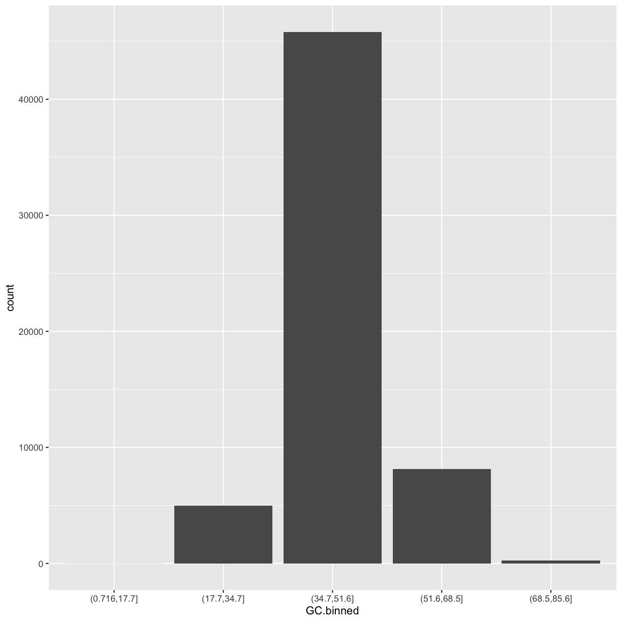
The bins created from cut() are useful in grouping data (a concept we often use in data analysis).
For example, we can use the GC.binned column to group data by %GC content bins to see how GC content
has an impact on other variables. To do this, we map aesthetics like color, fill, or linetype to our GC.binned column:
ggplot(data = dvst) + geom_density(mapping = aes(x=depth, linetype=GC.binned), alpha=0.5)
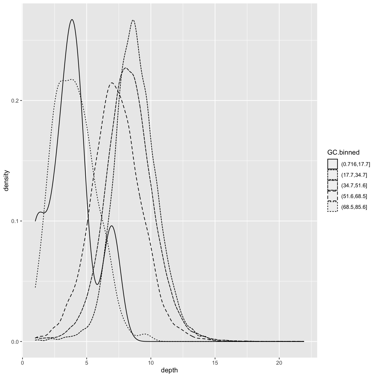
What happens if we geom_bar()’s x aesthetic is mapped to a continuous column (e.g., percent.GC)? geom_bar() will automatically bin the data itself, creating a histogram:
ggplot(data = dvst) + geom_bar(mapping = aes(x=percent.GC))
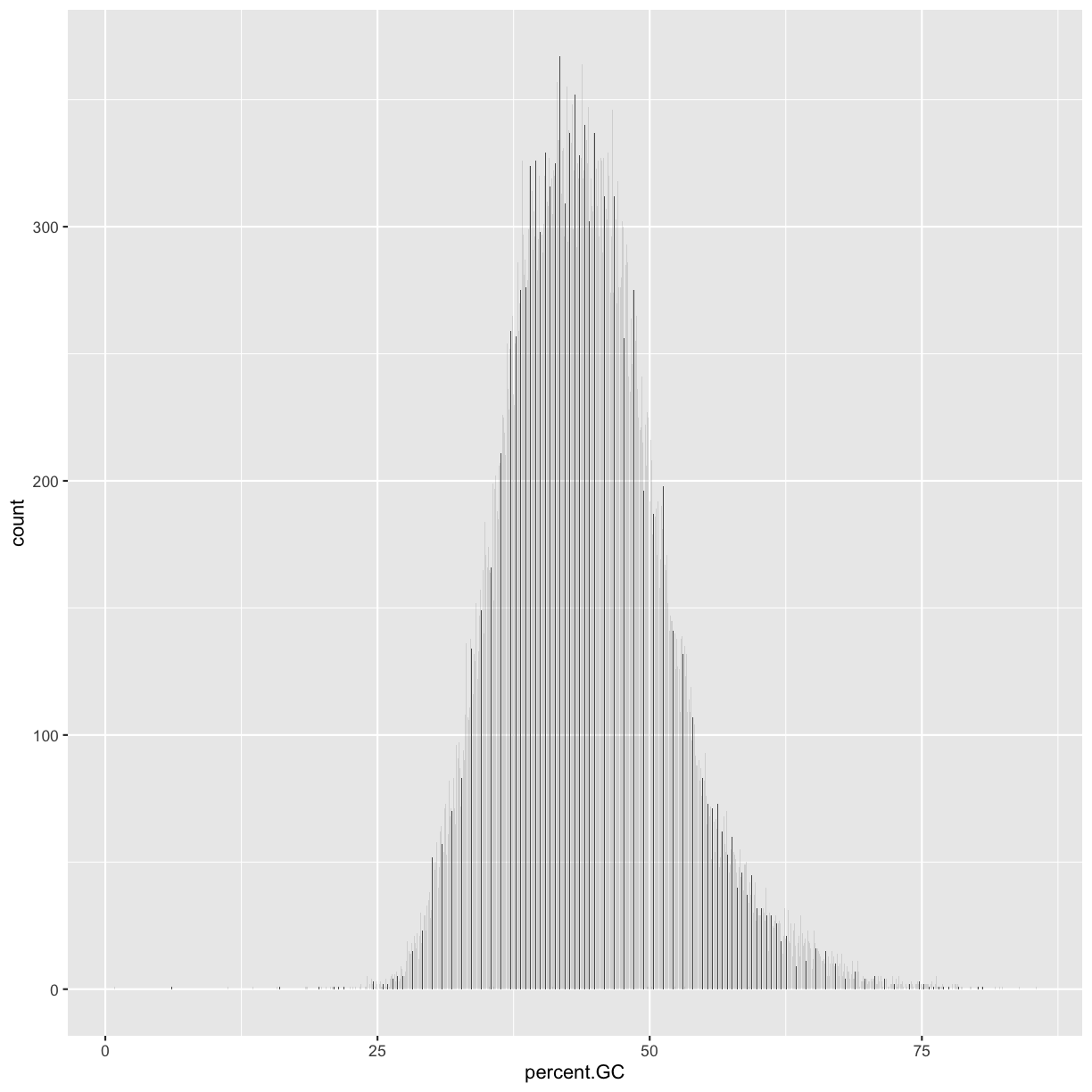
But it does not look like the plot we had! Hence, the challenge:
Challenge 3: Finding the Right Bin Width
We’ve seen before how different bin widths can drastically change the way we view and understand the data. Try creating a histogram of Pi with varying binwidths using:
ggplot(dvst) + geom_hist(aes(x=Pi), binwidth=1) + scale_x_continuous(limits=c(0.01, 80)). Using scale_x_continuous() just ignores all windows with 0 Pi and zooms into the figure. Try binwidths of 0.05, 0.5, 1, 5, and 10. What do you observe?Solution to challenge 3
Smaller bin widths can fit the data better (revealing more subtle details about the distribution), but there’s a trade-off. As bin widths become narrower, each bin will contain fewer data points and consequently be more noisy (and undersmoothed). Using wider bins smooth over this noise. However, bins that are too wide result in oversmoothing, which can hide details about the data.
Position adjustments
There’s one more piece of magic associated with bar charts. You can color a bar chart using
either the colour aesthetic, or, more usefully, fill:
ggplot(data = dvst) +
  geom_bar(mapping = aes(x = GC.binned, colour = GC.binned))
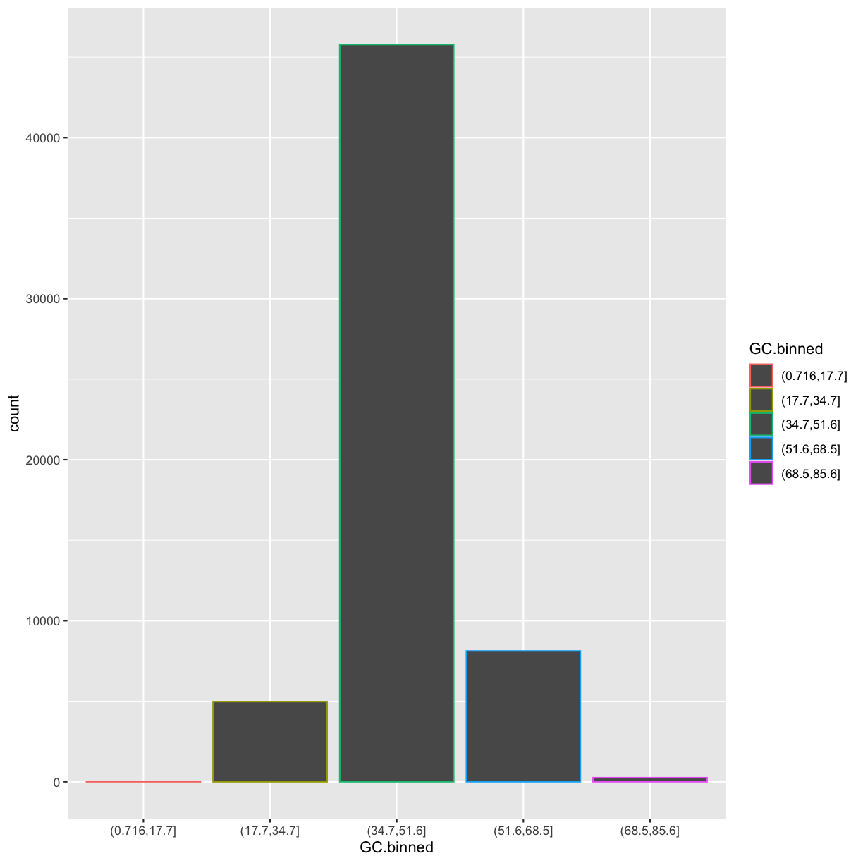
ggplot(data = dvst) +
  geom_bar(mapping = aes(x = GC.binned, fill = GC.binned))
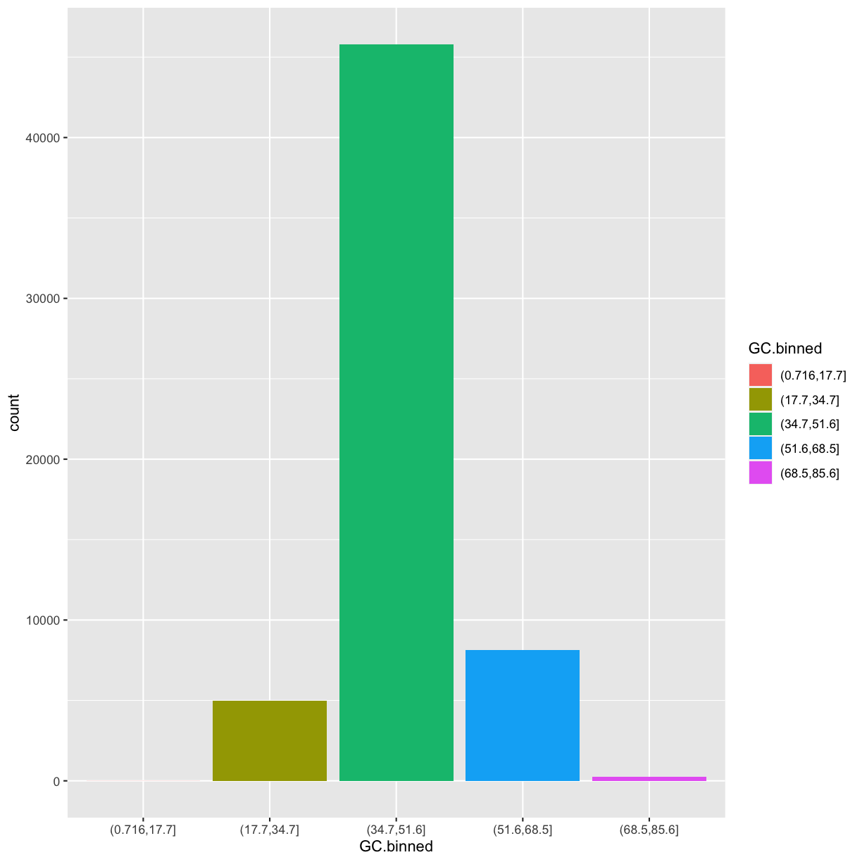
But what happen if you map the fill aesthetic to another variable, like cent? The bars are automatically stacked!
Each colored rectangle represents a combination of GC.binned and cent.
ggplot(data = dvst) +
  geom_bar(mapping = aes(x = GC.binned, fill = cent))
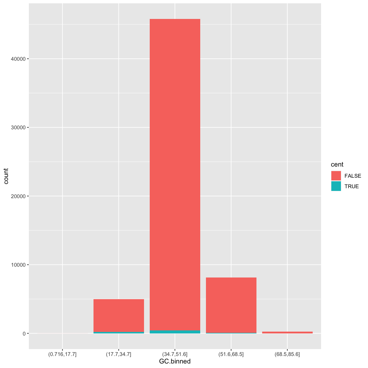
The stacking is performed automatically by the position adjustment specified by the position argument. If you don’t want a stacked bar chart, you can use one of three other options: "identity", "dodge" or "fill".
-
position = "identity"will place each object exactly where it falls in the context of the graph. This is not very useful for bars, because it overlaps them. However, the identity position adjustment is more useful for 2d geoms, like points, where it is the default. -
position = "fill"works like stacking, but makes each set of stacked bars the same height. This makes it easier to compare proportions across groups.ggplot(data = dvst) + geom_bar(mapping = aes(x = GC.binned, fill = cent), position = "fill")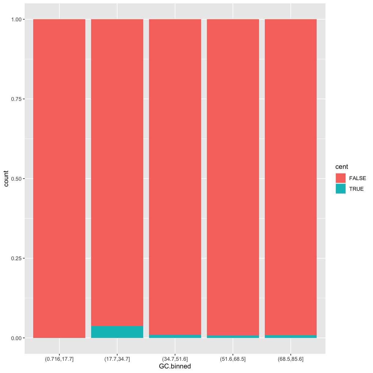
-
position = "dodge"places overlapping objects directly beside one another. This makes it easier to compare individual values.ggplot(data = dvst) + geom_bar(mapping = aes(x = GC.binned, fill = cent), position = "dodge")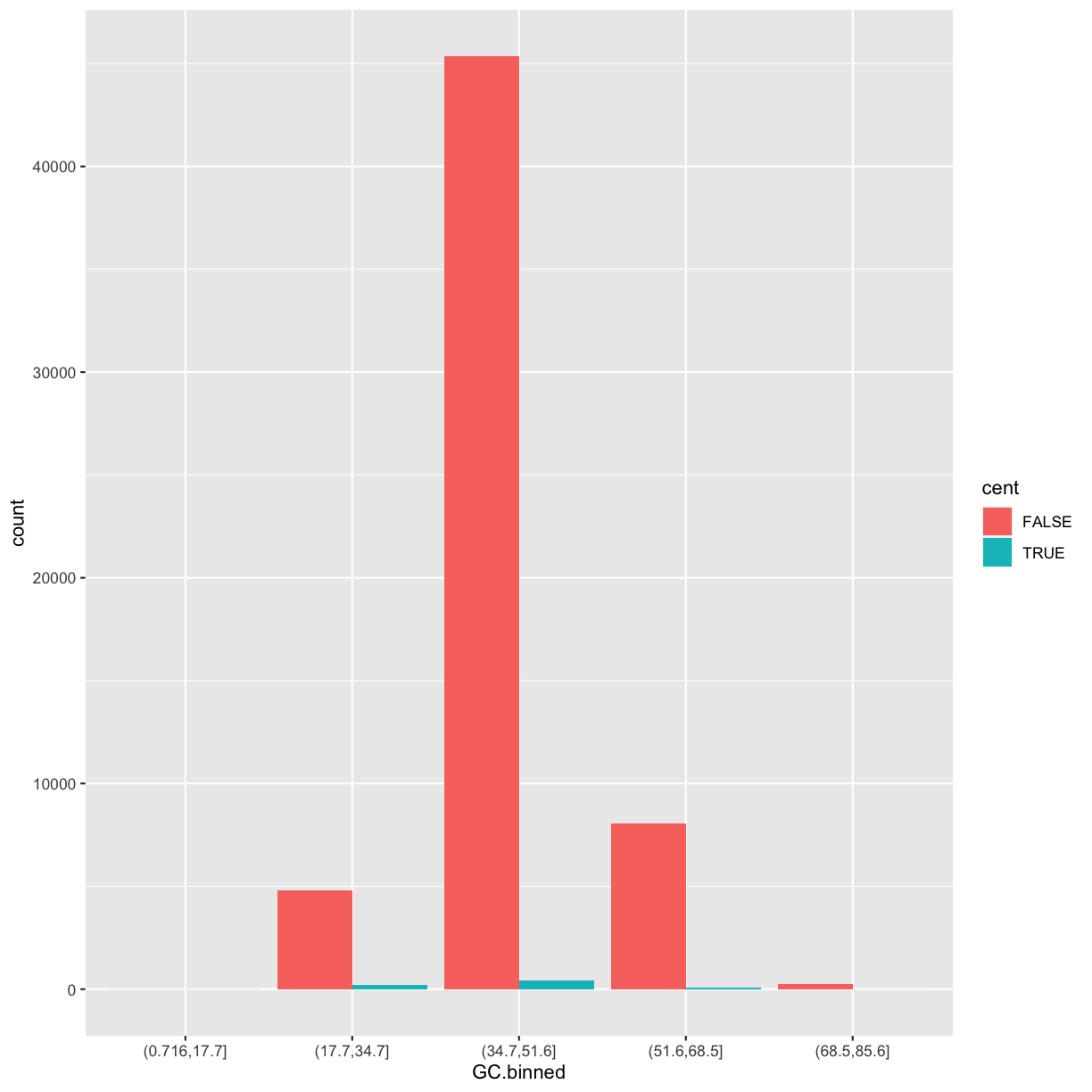
Dataset #2
Now we’ll return for a minute to data manipulation and create a new tbl by
merging two additional datasets available in Buffalo’s
bds-files GitHub repository for chapter 8. We start by reading these datasets
with read_tsv:
#Read datasets
mtfs <- read_tsv("https://raw.githubusercontent.com/vsbuffalo/bds-files/master/chapter-08-r/motif_recombrates.txt")
rpts <- read_tsv("https://raw.githubusercontent.com/vsbuffalo/bds-files/master/chapter-08-r/motif_repeats.txt")
Here is how they look like:
head(mtfs)
# A tibble: 6 x 9
  chr   motif_start motif_end   dist recomb_start recomb_end  recom motif  pos
  <chr>       <dbl>     <dbl>  <dbl>        <dbl>      <dbl>  <dbl> <chr>  <chr>
1 chrX     35471312  35471325 39323      35430651   35433340 0.0015 CCTCC… chrX…
2 chrX     35471312  35471325 36977      35433339   35435344 0.0015 CCTCC… chrX…
3 chrX     35471312  35471325 34798.     35435343   35437699 0.0015 CCTCC… chrX…
4 chrX     35471312  35471325 31850.     35437698   35441240 0.0015 CCTCC… chrX…
5 chrX     35471312  35471325 27463      35441239   35446472 0.0015 CCTCC… chrX…
6 chrX     35471312  35471325 24834      35446471   35446498 0.0016 CCTCC… chrX…
head(rpts)
# A tibble: 6 x 5
  chr       start       end name  motif_start
  <chr>     <dbl>     <dbl> <chr>       <dbl>
1 chrX   63005829  63006173 L2       63005830
2 chrX   67746983  67747478 L2       67747232
3 chrX  118646988 118647529 L2      118647199
4 chrX  123998417 123998701 L2      123998675
5 chr13  36171897  36172404 L2       36172069
6 chr13  47030437  47031075 L2       47030836
These two datasets come from a study that explored recombination rates around a degenerate sequence motif that is common in some repeat classes. The first dataset contains estimates of the recombination rate for all windows within 40kb of each of the two motif variants. The second dataset contains info about repeats each motif occur in. Our goal will be to merge these two datasets to look at the effect of specific repeat background on recombination rate.
Using ggplot2 Facets
Here is the plan:
- combine chr, and motif_start columns in
rptsas pos withunite, - select this new column along with the name column, and
- join these two columns with the columns in the
mtfswithinner_join. Note, there are several ways you can join to two dataframes.
#Combine columns
rpts2 <- rpts %>%
  unite(pos, chr, motif_start, sep="-") %>% ## new function!
  select(name, pos) %>%
  inner_join(mtfs, by="pos")
We will now explore these data using visualization technique known as facets. Facets allow us to visualize grouped data by creating a series of separate adjacent plots for each group. Let’s first glimpse at the relationship between recombination rate and distance to a motif. We’ll construct this graphic in steps:
p <- ggplot(data = rpts2, mapping = aes(x=dist, y=recom)) + geom_point(size=1)
p <- p + geom_smooth(method="loess", se=FALSE, span=1/10)
print(p)
`geom_smooth()` using formula 'y ~ x'
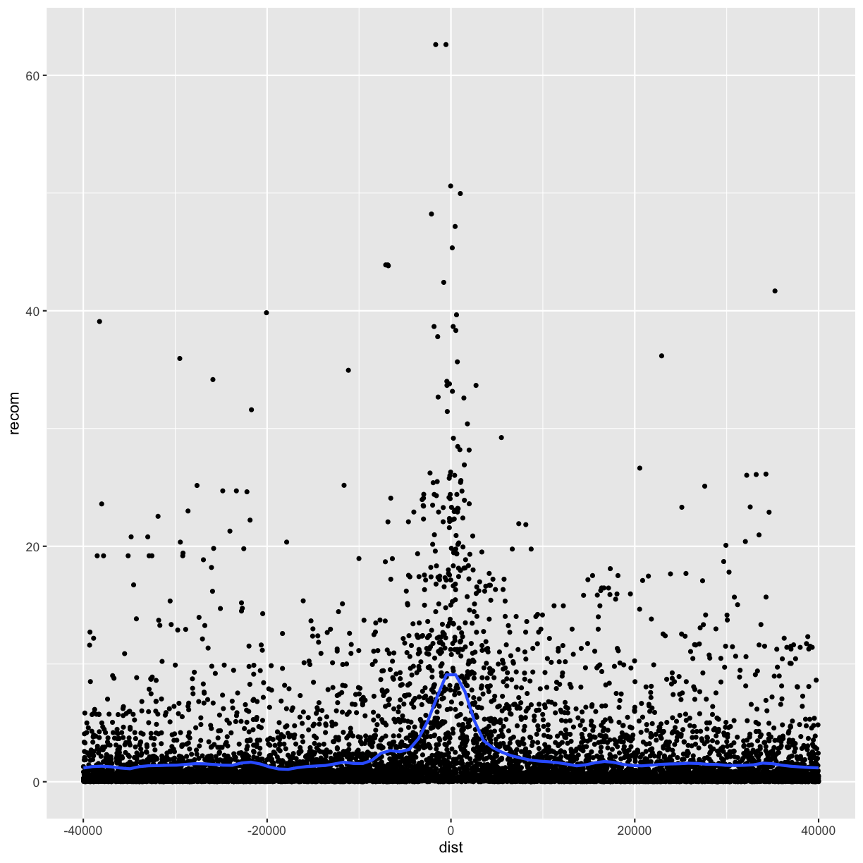
Note that we’ve turned off geom_smooth()’s standard error estimates,
adjusted the smoothing with span, and set the smoothing method to “loess”.
From this data, we only see a slight bump in the smoothing curve where the motifs reside. However, this data is a convolution of two different motif sequences on many different genomic backgrounds. In other words, there’s a large amount of heterogeneity we’re not accounting for, and this could be washing out our signal. Let’s use faceting to pick apart this data.
First, if you’ve explored the rpts dataframe, you’ll notice that the
motif column contains two variations of the sequence motif:
distinct(rpts2, motif)
# A tibble: 2 x 1
  motif
  <chr>
1 CCTCCCTGACCAC
2 CCTCCCTAGCCAC
One way to compare these is by grouping and coloring the loess curves by motif sequence:
ggplot(data = rpts2, mapping = aes(x=dist, y=recom)) + geom_point(size=1) +
  geom_smooth(aes(color=motif), method="loess", se=FALSE, span=1/10)
`geom_smooth()` using formula 'y ~ x'
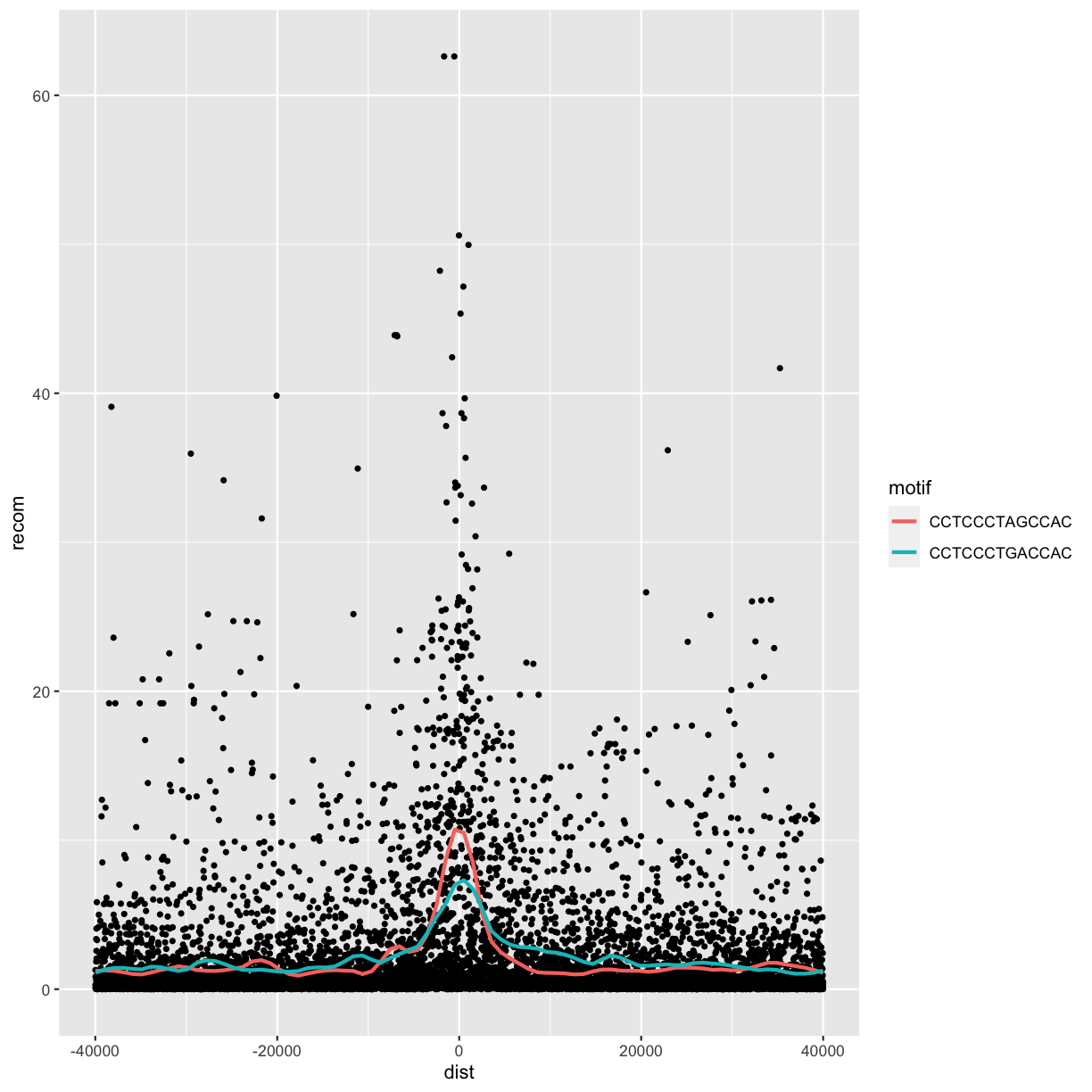
Alternatively, we can split these motifs apart visually with
facets using ggplot2’s facet_wrap() or facet_grid().
Facet_wrap()
To facet your plot by a single variable, use facet_wrap(). facet_wrap() takes a
factor column, creates a panel for each level and wraps around horizontally.
The first argument of facet_wrap() should be a formula, which you create with ~
followed by a variable name.
p <- ggplot(data = rpts2, mapping = aes(x=dist, y=recom)) + geom_point(size=1, color="grey")
p <- p + geom_smooth(method='loess', se=FALSE, span=1/10)
p <- p + facet_wrap(~ motif)
print(p)
`geom_smooth()` using formula 'y ~ x'
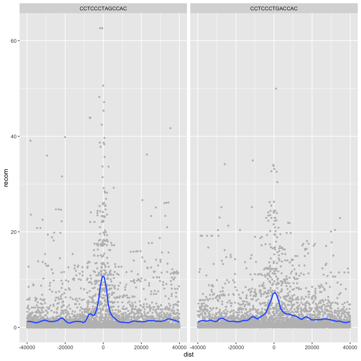
Facet_grid()
To facet your plot on the combination of two variables, add facet_grid() to your plot call.
The first argument of facet_grid() is also a formula. This time the formula should contain
two variable names separated by a ~.
If you prefer to not facet in the rows or columns dimension, use a . instead of a
variable name, e.g. + facet_grid(. ~ motif).
rpts
# A tibble: 317 x 5
   chr       start       end name  motif_start
   <chr>     <dbl>     <dbl> <chr>       <dbl>
 1 chrX   63005829  63006173 L2       63005830
 2 chrX   67746983  67747478 L2       67747232
 3 chrX  118646988 118647529 L2      118647199
 4 chrX  123998417 123998701 L2      123998675
 5 chr13  36171897  36172404 L2       36172069
 6 chr13  47030437  47031075 L2       47030836
 7 chr13 112828064 112828466 L2      112828268
 8 chr12  44799399  44799664 L2       44799602
 9 chr12  71407097  71407379 L2       71407292
10 chr12 102646349 102646646 L2      102646586
# … with 307 more rows
p <- ggplot(rpts2, aes(x=dist, y=recom)) + geom_point(size=1, color="grey")
p <- p + geom_smooth(method='loess', se=FALSE, span=1/16)
p <- p + facet_grid(name ~ motif)
print(p)
`geom_smooth()` using formula 'y ~ x'
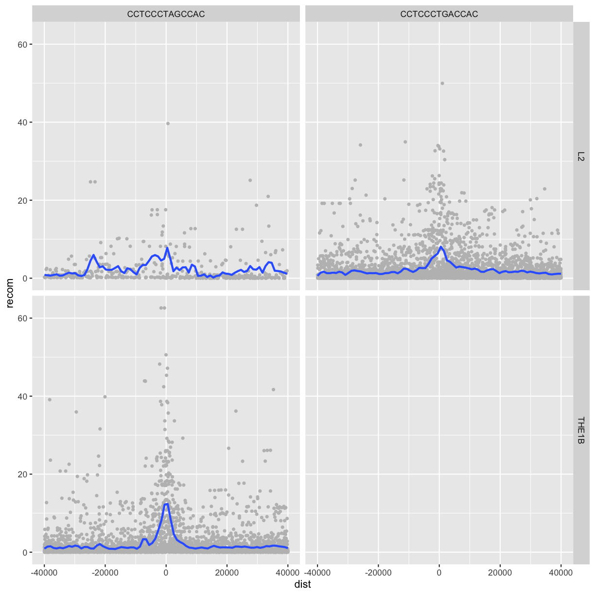
We see some patterns emerging here: motif CCTCCCTAGCCAC on a THE1B repeat background has a strong effect on recombination rate, as does CCTCCCTGACCAC on a L2 repeat background. You can get a sense of the data that goes into this plot with:
table(rpts2$name, rpts2$motif, useNA="ifany")
        CCTCCCTAGCCAC CCTCCCTGACCAC
  L2              457          4110
  THE1B          4651             0
rpts2 %>%
  count(name, motif)
# A tibble: 3 x 3
  name  motif             n
  <chr> <chr>         <int>
1 L2    CCTCCCTAGCCAC   457
2 L2    CCTCCCTGACCAC  4110
3 THE1B CCTCCCTAGCCAC  4651
One important feature of facet_wrap() and facet_grid()
is that by default, x- and y-scales will be the same across
all panels. You can set scales to be free with scales=”free_x”
and scales=”free_y”, or scales=”free” to free both axes.
For example:
p <- ggplot(rpts2, aes(x=dist, y=recom)) + geom_point(size=1, color="grey")
p <- p + geom_smooth(method='loess', se=FALSE, span=1/10)
p <- p + facet_wrap( ~ motif, scales="free_y")
print(p)
`geom_smooth()` using formula 'y ~ x'
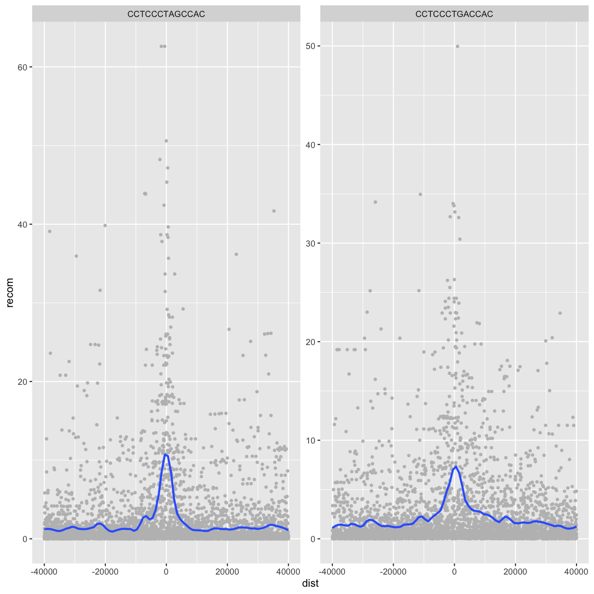
Challenge 4: Recombination rate by chromosome
Try using facets to look at this data when grouped by chromosome with facet_wrap( ~ chr).
Extra reading: coordinate systems
Coordinate systems are probably the most complicated part of ggplot2. The default coordinate system is the Cartesian coordinate system where the x and y positions act independently to determine the location of each point. There are a number of other coordinate systems that are occasionally helpful.
coord_flip()switches the x and y axes. This is useful (for example), if you want horizontal boxplots. It’s also useful for long labels: it’s hard to get them to fit without overlapping on the x-axis.#fig.width = 3, out.width = "50%", fig.align = "default"} ggplot(data = mpg, mapping = aes(x = class, y = hwy)) + geom_boxplot()
ggplot(data = mpg, mapping = aes(x = class, y = hwy)) +
  geom_boxplot() +
  coord_flip()
coord_quickmap()sets the aspect ratio correctly for maps. This is very important if you’re plotting spatial data with ggplot2.#fig.width = 3, out.width = "50%", fig.align = "default", message = FALSE} nz <- map_data("nz")Error: Package `maps` required for `map_data`. Please install and try again.ggplot(nz, aes(long, lat, group = group)) + geom_polygon(fill = "white", colour = "black")Error in ggplot(nz, aes(long, lat, group = group)): object 'nz' not foundggplot(nz, aes(long, lat, group = group)) + geom_polygon(fill = "white", colour = "black") + coord_quickmap()Error in ggplot(nz, aes(long, lat, group = group)): object 'nz' not found
coord_polar()uses polar coordinates. Polar coordinates reveal an interesting connection between a bar chart and a Coxcomb chart.#fig.width = 3, out.width = "50%", fig.align = "default", fig.asp = 1} bar <- ggplot(data = diamonds) + geom_bar( mapping = aes(x = cut, fill = cut), show.legend = FALSE, width = 1 ) + theme(aspect.ratio = 1) + labs(x = NULL, y = NULL) bar + coord_flip()
bar + coord_polar()
Saving the plot
ggsave() is a convenient function for saving a plot. It defaults to saving the last plot that you displayed, using the size of the current graphics device. It also guesses the type of graphics device from the extension.
ggsave("myplot.pdf")
ggsave("myplot.png")
The layered grammar of graphics
In the previous sections, you learned much more than how to make scatterplots, bar charts, and boxplots. You learned a foundation that you can use to make any type of plot with ggplot2. To see this, let’s add position adjustments, stats, coordinate systems, and faceting to our code template:
ggplot(data = <DATA>) +
  <GEOM_FUNCTION>(
     mapping = aes(<MAPPINGS>),
     stat = <STAT>,
     position = <POSITION>
  ) +
  <COORDINATE_FUNCTION> +
  <FACET_FUNCTION>
Our new template takes seven parameters, the bracketed words that appear in the template. In practice, you rarely need to supply all seven parameters to make a graph because ggplot2 will provide useful defaults for everything except the data, the mappings, and the geom function.
The seven parameters in the template compose the grammar of graphics, a formal system for building plots. The grammar of graphics is based on the insight that you can uniquely describe any plot as a combination of a dataset, a geom, a set of mappings, a stat, a position adjustment, a coordinate system, and a faceting scheme.
You could use this method to build any plot that you imagine. In other words, you can use the code template that you’ve learned in this chapter to build hundreds of thousands of unique plots.
ggplot2 calls
So far we’ve been very explicit with ggplot2 code:
ggplot(data = faithful, mapping = aes(x = eruptions)) +
  geom_freqpoly(binwidth = 0.25)
Typically, the first one or two arguments to a function are so important that you should know them by heart. The first two arguments to ggplot() are data and mapping, and the first two arguments to aes() are x and y. And if you know them by heart, you don’t need to type them! That makes it easier to see what’s different between plots. Rewriting the previous plot more concisely yields:
ggplot(faithful, aes(eruptions)) +
  geom_freqpoly(binwidth = 0.25)
Sometimes we’ll turn the end of a pipeline of data transformation into a plot.
Watch for the transition from %>% to +. This transition is necessary because
ggplot2 was created before the pipe was discovered.
Key Points
Use
ggplot2to create plots.Think about graphics in layers: aesthetics, geometry, statistics, scale transformation, and grouping.
Writing and Applying Functions to Data
Overview
Teaching: 20 min
Exercises: 10 minQuestions
What are
applyfunctions in R?How can I write a new function in R?
Objectives
Define a function that takes arguments.
Return a value from a function.
Test a function.
Set default values for function arguments.
Explain why we should divide programs into small, single-purpose functions.
Writing and Applying Functions to Data
In this section, we’ll cover one of the cornerstones of R: how to write and apply functions to data.
This approach of applying functions to data rather than writing explicit loops follows from a
functional-programming style that R inherited from one of its language influences, Scheme.
Specifically, our focus will be on applying functions to R’s lists using lapply() and sapply(), but
the same ideas extend to other R data structures through similar “apply” functions. Solving common
data analysis problems with apply functions is tricky at first, but mastering it will serve you well in R.
Using lapply() with lists
Suppose you have a list of numeric values (here, generated at random with rnorm()):
ll <- list(a=rnorm(6, mean=1), b=rnorm(6, mean=4), c=rnorm(6, mean=6))
ll
$a
[1]  0.5328209  1.2479357 -0.5604071  0.7299258  0.8129378  2.1838192

$b
[1] 4.816460 4.220313 3.931735 4.978639 2.946376 4.851820

$c
[1] 7.626979 5.586155 5.206131 6.694440 4.559841 5.406048
How might we calculate the mean of each vector stored in this list? If you’re familiar with for loops in other languages, you may approach this problem using R’s for loops:
for (i in 1:length(ll)) {
  print(mean(ll[[i]]))
}
[1] 0.8245054
[1] 4.290891
[1] 5.846599
However, this is not idiomatic R; a better approach is to use an apply function that applies another function to each list element.
Apply functions
Function Description Example apply apply a function to a matrix apply(x, margin, function)lapply apply a function to a list; return a list lapply(list, sum)sapply same as lapply, but returns a vectorsapply(list, sum)tapply apply a function to a vector split based on factor levels tapply(mtcars$wt, mtcars$cyl, mean)vapply same as sapplybut you need to specify the type of return valuevapply(list, sum, FUN.VALUE=double(1))mapply a multivariate version of sapply mapply(rep, 1:4, 4:1)margin = 1 indicates rows, margin = 2 indicates columns
For example,
to calculate the mean of each list element, we’d want to apply the function mean() to each element. To do so,
we can use the function lapply() (the l is for list):
lapply(ll, mean)
$a
[1] 0.8245054

$b
[1] 4.290891

$c
[1] 5.846599
lapply() has several advantages over the loop shown above:
- it creates the output list for us,
- uses fewer lines of code,
- leads to clearer code, and
- is usually faster than using a for loop.
We can also use lapply() in parallel (see p. 233 of the textbook for details)
Tips for
applyfunctions1) Don’t call the function you pass to lapply()—for example, don’t do
lapply(ll, mean(x))or `lapply(ll, mean()).2) In some cases you will need to specify additional arguments to the function you’re passing to
lapply(). For example, mean() returns NA if some data are missing. We ignore NA values by callingmean()with the argumentna.rm=TRUE:ll[[c(3,2)]] <- NA lapply(ll, mean)$a [1] 0.8245054 $b [1] 4.290891 $c [1] NAll[[c(3,2)]] <- NA lapply(ll, mean, na.rm=TRUE)$a [1] 0.8245054 $b [1] 4.290891 $c [1] 5.898688
Writing functions.
Sometimes, we don’t have an exact function that we want to apply to our data. But we can just write it :) R makes writing functions very easy, both because you should be writing lots of them to organize your code and applying functions is such a common operation in R.
What is a function?
Functions gather a sequence of operations into a whole, preserving it for ongoing use. Functions provide:
- a name we can remember and invoke it by
- relief from the need to remember the individual operations
- a defined set of inputs and expected outputs
- rich connections to the larger programming environment
As the basic building block of most programming languages, user-defined functions constitute “programming” as much as any single abstraction can. If you have written a function, you are a computer programmer.
For example, we could write a simple version of R’s mean() function with na.rm=TRUE and apply it to the list:
meanRemoveNA <- function(x) mean(x, na.rm=TRUE)
lapply(ll, meanRemoveNA)
$a
[1] 0.8245054

$b
[1] 4.290891

$c
[1] 5.898688
The syntax for meanRemoveNA() is a common shortened version of the general syntax for R functions:
fun_name <- function(args) {
# body, containing R expressions
return(value)
}
Function definitions consist of arguments, a body, and a return value. Functions that contain only one line
in their body can omit the braces (as the meanRemoveNA() function does). Similarly, using return() to specify
the return value is optional; R’s functions will automatically return the last evaluated expression in the body.
These syntactic shortcuts are commonly used in R, as we often need to quickly write functions to apply to data.
Alternatively, we could forgo creating a function named meanRemoveNA() in our global environment altogether
and instead use an anonymous function. Anonymous functions are useful when we only need a function once for
a specific task:
lapply(ll, function(x) mean(x, na.rm=TRUE))
$a
[1] 0.8245054

$b
[1] 4.290891

$c
[1] 5.898688
meanRemoveNAVerbose <- function(x, warn=TRUE) {
# A function that removes missing values when calculating the mean # and warns us about it.
if (any(is.na(x)) && warn) { warning("removing some missing values!")
}
mean(x, na.rm=TRUE)
}
lapply(ll, meanRemoveNAVerbose)
Warning in FUN(X[[i]], ...): removing some missing values!
$a
[1] 0.8245054

$b
[1] 4.290891

$c
[1] 5.898688
Note, that functions over one line should be kept in a file and sent to the interpreter. RStudio conveniently allows you to send a whole function definition at once with Command-Option-f on a Mac and Control-Alt-f on Windows.
If you’ve been writing these functions down into a separate R script
(a good idea!), you can load in the functions into our R session by using the
source function:
source("functions/functions-lesson.R")
Function tips
Pass by value
Functions in R almost always make copies of the data to operate on inside of a function body. When we modify these data inside the function we are modifying the copy of them, not the original variable we gave as the first argument.
This is called “pass-by-value” and it makes writing code much safer: you can always be sure that whatever changes you make within the body of the function, stay inside the body of the function.
Function scope
Another important concept is scoping: any variables (or functions!) you create or modify inside the body of a function only exist for the lifetime of the function’s execution. Even if we have variables of the same name in our interactive R session, they are not modified in any way when executing a function.
Additional resources
R has some unique aspects that can be exploited when performing more complicated operations. We will not be writing anything that requires knowledge of these more advanced concepts. In the future when you are comfortable writing functions in R, you can learn more by reading the R Language Manual or this chapter from Advanced R Programming by Hadley Wickham. For context, R uses the terminology “environments” instead of frames.
Tip4: Testing and documenting
It’s important to both test functions and document them: Documentation helps you, and others, understand what the purpose of your function is, and how to use it, and its important to make sure that your function actually does what you think.
When you first start out, your workflow will probably look a lot like this:
- Write a function
- Comment parts of the function to document its behaviour
- Load in the source file
- Experiment with it in the console to make sure it behaves as you expect
- Make any necessary bug fixes
- Rinse and repeat.
Formal documentation for functions, written in separate
.Rdfiles, gets turned into the documentation you see in help files. The [roxygen2][roxygen] package allows R coders to write documentation alongside the function code and then process it into the appropriate.Rdfiles. You will want to switch to this more formal method of writing documentation when you start writing more complicated R projects.Formal automated tests can be written using the testthat package.
Key Points
Use
functionto define a new function in R.Use parameters to pass values into functions.
Load functions into programs using
source.
Developing Workflows with R Scripts
Overview
Teaching: 45 min
Exercises: 20 minQuestions
How can I make data-dependent choices in R?
How can I repeat operations in R?
Objectives
Write conditional statements with
if()andelse().Write and understand
for()loops.
Developing Workflows with R Scripts
Control Flow: if, for, and while
Often we want to control the flow of our actions. This can be done by setting actions to occur only if a condition or a set of conditions are met. Alternatively, we can also set an action to occur a particular number of times.
Three common control flow and looping statments are if, for, and while:
# if
if (x == some_value) {
            # do some stuff in here
} else if (x == other_value) {
            # elseif is optional
} else {
            #else is optional
}

#for
for (element in some_vector) {
            # iteration happens here
}

#while
while (something_is_true) {
            # do some stuff
}
You can break out of for and while loops with a break statement, and advance loops to the next iteration with next.
Examples:
# sample a random number from a Poisson distribution
# with a mean (lambda) of 8

x <- rpois(1, lambda=8)

if (x >= 10) {
  print("x is greater than or equal to 10")
}
x
[1] 8
Tip: pseudo-random numbers
In the above case, the function
rpois()generates a random number following a Poisson distribution with a mean (i.e. lambda) of 8. We can use functionset.seed()guarantees that all machines will generate the exact same ‘pseudo-random’ number (more about pseudo-random numbers).
for(i in 1:10){
  print(i)
}
[1] 1
[1] 2
[1] 3
[1] 4
[1] 5
[1] 6
[1] 7
[1] 8
[1] 9
[1] 10
for(i in 1:3){
  for(j in c('a', 'b', 'c')){
    print(paste(i,j))
  }
}
[1] "1 a"
[1] "1 b"
[1] "1 c"
[1] "2 a"
[1] "2 b"
[1] "2 c"
[1] "3 a"
[1] "3 b"
[1] "3 c"
z <- 1
while(z > 0.1){
  z <- runif(1)
  print(z)
}
[1] 0.3067685
[1] 0.4269077
[1] 0.6931021
[1] 0.08513597
ifelse
R also has a vectorized version of if: the ifelse function. Rather than control program flow, ifelse(test, yes, no)
returns the yes value for all TRUE cases of test, and no for all FALSE cases. For example:
x <-c(-3,1,-5,2)
ifelse(x < 0, -1, 1)
[1] -1 1 -1 1
Note, that although ifelse() is readable and clear, it can be slower than the following:
x <- c(-3, 1, -5, 2)
y <- rep(1, length(x))
y[x < 0] <- -1
y
[1] -1 1 -1 1
Pre-allocating vectors
One point worth mentioning is that if you do need to loop over a structure with a
fororwhileloop, always preallocate your results vector. You can create empty numeric vectors withnumeric(len)and empty integer vectors withinteger(len), wherelenis the length. For example, if you were to loop over two vectors to sum their values pairwise, do not use:x <- rnorm(10) y <- rnorm(10) res <- NULL for (i in 1:length(x)) { res <- c(res, x[i] + y[i]) }First, this is completely unecessary since we could calculate this with
res <-
x + y
. Second, this code would be needlessly slow because appending to vectors withres <- c(res, ...)is extremely computationally expensive in R.R’s vectors are allocated in memory to the exact length that the need to be. So each iteration of the above code requires (1) allocating a new
resvector one element longer, and (2) copying all ofres’s current elements over to this new vector.The correct way to do this (assuming in your real code something in the
forloop can’t be parallelized!) is:x <- rnorm(10) y <- rnorm(10) res <- numeric(10) # preallocation! for (i in 1:length(x)) { res[i] <- x[i] + y[i] }
Working with R Scripts
Although we’ve used R interactively, in practice your analyses should be kept in scripts that can be run many times throughout development. Scripts can be organized into project directories and checked into Git repositories. There’s also a host of excellent R tools (e.g., Knitr and Rmarkdown) to help in creating well-documented, reproducible projects in R.
You can run R scripts from R using the function source(). For example, to execute an R script named my_analysis.R
use:
source("my_analysis.R")
Alternatively, we can execute a script in batch mode from the command line with:
Rscript --vanilla my_analysis.R
This comes in handy when you need to rerun an analysis on different files or with different arguments
provided on the command line. It’s a good practice to use –vanilla option because by default, Rscript
will restore any past saved environments and save its current environment after the execution completes.
Usually we don’t want R to restore any past state from previous runs, as this can lead to irreproducible
results. Additionally, saved environments can make it a nightmare to debug a script. See R --help for
more information.
Lastly, if you want to retrieve command-line arguments passed to your script, use R’s commandArgs() with trailingOnly=TRUE. For example, this simple R script just prints all arguments:
echo "## args.R -- a simple script to show command line args
args <- commandArgs(TRUE)
print(args)" > args.R
We run this with:
Rscript --vanilla args.R arg1 arg2 arg3
[1] "arg1" "arg2" "arg3"
Working directory
It’s important to mind R’s working directory when writing scripts. Scripts should not use
setwd()to set their working directory, as this is not portable to other systems (which won’t have the same directory structure). For the same reason, use relative paths like ../data/achievers.txt when loading in data, and not absolute paths like /Users/jlebowski/data/achievers.txt. Also, it’s a good idea to indicate (either in comments or a README file) which directory the user should set as their working directory.
Workflows for Loading and Combining Multiple Files
See pages 257-260 of the book if you need to load and combine multiple files
Exporting Data
At some point during an analysis, you’ll need to export data from R. We can export dataframes to plain-text files
using the R function write.table(). Unfortunately, write.table() has some poorly chosen defaults that we usually
need to adjust. For example, if we wanted to write our dataframe mtfs to a tab-delimited file named hotspot_motifs.txt,
we would use:
write.table(mtfs, file="hotspot_motifs.txt", quote=FALSE, sep="\t", row.names=FALSE, col.names=TRUE)
write.table()’s first two arguments are the dataframe (or matrix) to write to file and the file path to save it to.
By default, write.table() quotes factor and character columns and includes rownames. We disable these with quote=FALSE and row.names=FALSE. We also can set the column separators to tabs with the sep argument. A header can be included or excluded with the col.names argument.
Given that many Unix tools work well with Gzipped files, it may be useful to write a compressed version of a
file directly from R. In addition to a string file path, write.table’s file argument also handles open file
connections. So to write our dataframe to a compressed file, we can open a gzipped file connect with gzfile():
hs_gzf <- gzfile("hotspot_motifs.txt.gz")
write.table(mtfs, file=hs_gzf, quote=FALSE, sep="\t", row.names=FALSE, col.names=TRUE)
While plain-text formats are the preferable way to share tabular datasets, it’s not the best way to save
complex R data structures like lists or special R objects. In these cases, it’s usually preferable to save R
objects as R objects. Encoding and saving objects to disk in a way that allows them to be restored as the original
object is known as serialization. R’s functions for saving and loading R objects are save() and load().
tmp <- list(vec=rnorm(4), df=data.frame(a=1:3, b=3:5))
save(tmp, file="example.Rdata")
rm(tmp) # remove the original 'tmp' list
load("example.Rdata") # this fully restores the 'tmp' list from file
str(tmp)
List of 2
 $ vec: num [1:4] -2.061 -0.6 -0.954 0.558
 $ df :'data.frame':	3 obs. of  2 variables:
  ..$ a: int [1:3] 1 2 3
  ..$ b: int [1:3] 3 4 5
The function save() has an analogous function called save.image() that saves all objects in your workspace
rather than just the objects you specify. Combined with savehistory(), save.image() can be a quick way to store
your past work in R in a rush.
Key Points
Use
ifandelseto make choices.Use
forto repeat operations.
Data Import
Overview
Teaching: 20 min
Exercises: 10 minQuestions
How to read data in R?
What are some potential problems with reading data in R?
How to write data in files?
Objectives
To understand how to read data into R
To learn most commonly used functions in
readrfor reading the filesTo understand and be able to fix common problems in reading data files
To know how to write data into a file
Data import

Introduction
Before transforming data we have to learn how to read them into R. We’ll start by learning how to read plain-text rectangular files into R. We’ll finish with a few pointers to packages that are useful for other types of data.
The tutorial is based on Chapter 10 of the R for Data Science book by Garrett Grolemund and Hadley Wickham. Check this book for more details.
Prerequisites
We’ll be using package readr to load flat files into R. This packages is a part of the core tidyverse, an “an opinionated collection of R packages designed for data science”.
if (!require("tidyverse")) install.packages("tidyverse")
library(tidyverse)
Getting started
The four most commonly used functions in readr are read_csv, read_csv2, read_tsv, and read_delim.
read_csv()reads comma delimited files,read_csv2()reads semicolon separated files (common in countries where,is used as the decimal place),read_tsv()reads tab delimited files, andread_delim()reads in files with any delimiter.
These functions all have similar syntax; we will use read_csv as an example.
The first argument to read_csv() is the to the file to read.
heights <- read_csv("../data/heights.csv")
Error: '../data/heights.csv' does not exist in current working directory ('/Users/dlavrov/GitHub/Teaching/BCB546-all/BCB546-R/_episodes_rmd').
When you run read_csv() it prints out a column specification that gives the name and type of each column.
You can also supply an inline csv file. This is useful for experimenting with readr and for creating reproducible examples to share with others:
read_csv("a,b,c
1,2,3
4,5,6")
# A tibble: 2 x 3
      a     b     c
  <dbl> <dbl> <dbl>
1     1     2     3
2     4     5     6
In both cases read_csv() uses the first line of the data for the column names, which is a very common convention. There are two cases where you might want to tweak this behaviour:
-
Sometimes there are a few lines of metadata at the top of the file. You can use
skip = nto skip the firstnlines; or usecomment = "#"to drop all lines that start with (e.g.)#.read_csv("The first line of metadata The second line of metadata x,y,z 1,2,3", skip = 2)# A tibble: 1 x 3 x y z <dbl> <dbl> <dbl> 1 1 2 3read_csv("# A comment I want to skip x,y,z 1,2,3", comment = "#")# A tibble: 1 x 3 x y z <dbl> <dbl> <dbl> 1 1 2 3 -
The data might not have column names. You can use
col_names = FALSEto tellread_csv()not to treat the first row as headings, and instead label them sequentially fromX1toXn. Alternatively you can passcol_namesa character vector which will be used as the column names:read_csv("1,2,3\n4,5,6", col_names = c("x", "y", "z"))# A tibble: 2 x 3 x y z <dbl> <dbl> <dbl> 1 1 2 3 2 4 5 6
Another option that commonly needs tweaking is na: this specifies the value (or values)
that are used to represent missing values in your file:
read_csv("a,b,c\n1,2,.", na = ".")
# A tibble: 1 x 3
      a     b c
  <dbl> <dbl> <lgl>
1     1     2 NA
Compared to base R
If you’ve used R before, you might wonder why we’re not using read.csv().
There are a few good reasons to favour readr functions over the base equivalents:
-
They are typically much faster (~10x) than their base equivalents. There is even a faster version,
data.table::fread(), but it doesn’t fit quite so well into the tidyverse. -
They produce tibbles, they don’t convert character vectors to factors, use row names, or munge the column names. These are common sources of frustration with the base R functions.
-
They are more reproducible. Base R functions inherit some behaviour from your operating system and environment variables, so import code that works on your computer might not work on someone else’s.
Writing to a file
readr also comes with two useful functions for writing data back to disk: write_csv() and write_tsv().
Both functions increase the chances of the output file being read back in correctly by:
-
Always encoding strings in UTF-8.
-
Saving dates and date-times in ISO8601 format so they are easily parsed elsewhere.
If you want to export a csv file to Excel, use write_excel_csv() — this writes a special character
(a “byte order mark”) at the start of the file which tells Excel that you’re using the UTF-8 encoding.
The most important arguments are x (the data frame to save), and path (the location to save it).
You can also specify how missing values are written with na, and if you want to append to an existing file.
write_csv(challenge, "challenge.csv")
Note that the type information is lost when you save to csv:
challenge
# A tibble: 2,000 x 2
       x y
   <dbl> <date>
 1   404 NA
 2  4172 NA
 3  3004 NA
 4   787 NA
 5    37 NA
 6  2332 NA
 7  2489 NA
 8  1449 NA
 9  3665 NA
10  3863 NA
# … with 1,990 more rows
write_csv(challenge, "challenge-2.csv")
read_csv("challenge-2.csv")
── Column specification ─────────────────────────────────────────────────────────────────────────────────────────────────────────────────────────────────────────────────────────────────────────────────────
cols(
  x = col_double(),
  y = col_logical()
)
# A tibble: 2,000 x 2
       x y
   <dbl> <lgl>
 1   404 NA
 2  4172 NA
 3  3004 NA
 4   787 NA
 5    37 NA
 6  2332 NA
 7  2489 NA
 8  1449 NA
 9  3665 NA
10  3863 NA
# … with 1,990 more rows
This makes CSVs a little unreliable for caching interim results—you need to recreate the column specification every time you load in. There are two alternatives:
-
write_rds()andread_rds()are uniform wrappers around the base functionsreadRDS()andsaveRDS(). These store data in R’s custom binary format called RDS:write_rds(challenge, "challenge.rds") read_rds("challenge.rds")# A tibble: 2,000 x 2 x y <dbl> <date> 1 404 NA 2 4172 NA 3 3004 NA 4 787 NA 5 37 NA 6 2332 NA 7 2489 NA 8 1449 NA 9 3665 NA 10 3863 NA # … with 1,990 more rows -
The feather package implements a fast binary file format that can be shared across programming languages:
library(feather)
write_feather(challenge, "challenge.feather")
read_feather("challenge.feather")
#> # A tibble: 2,000 x 2
#>       x      y
#>   <dbl> <date>
#> 1   404   <NA>
#> 2  4172   <NA>
#> 3  3004   <NA>
#> 4   787   <NA>
#> 5    37   <NA>
#> 6  2332   <NA>
#> # ... with 1,994 more rows
Feather tends to be faster than RDS and is usable outside of R. However, RDS supports list-columns while feather currently does not.
Other types of data
To get other types of data into R, we recommend starting with the tidyverse packages listed below. They’re certainly not perfect, but they are a good place to start. For rectangular data:
-
haven reads SPSS, Stata, and SAS files.
-
readxl reads excel files (both
.xlsand.xlsx). -
DBI, along with a database specific backend (e.g. RMySQL, RSQLite, RPostgreSQL etc) allows you to run SQL queries against a database and return a data frame.
For hierarchical data: use jsonlite (by Jeroen Ooms) for json, and xml2 for XML. Jenny Bryan has some excellent worked examples at https://jennybc.github.io/purrr-tutorial/.
For other file types, try the R data import/export manual and the rio package.
Homework
Parse the UNIX assignment files (fang_et_al_genotypes.txt and snp_position.txt) into R.
- What problems did you encounter?
- Did R guessed the data type correctly?
- If not, how did you fix it?
Try to use the
tfunction to transpose the first file
- Did it work?
- Can you figure out how to make it work?
Parsing a vector (read if you run into problems or if like details)
Before we get into the details of how readr reads files from disk, we need to take a little
detour to talk about the parse_*() functions. These functions take a character vector and
return a more specialised vector like a logical, integer, or date. These functions are useful
in their own right, but are also an important building block for readr. Like all functions
in the tidyverse, the parse_*() functions are uniform: the first argument is a character
vector to parse, and the na argument specifies which strings should be treated as missing:
parse_integer(c("1", "231", ".", "456"), na = ".")
[1] 1 231 NA 456
If parsing fails, you’ll get a warning:
x <- parse_integer(c("123", "345", "abc", "123.45"))
Warning: 2 parsing failures.
row col               expected actual
  3  -- an integer             abc
  4  -- no trailing characters 123.45
And the failures will be missing in the output:
x
[1] 123 345  NA  NA
attr(,"problems")
# A tibble: 2 x 4
    row   col expected               actual
  <int> <int> <chr>                  <chr>
1     3    NA an integer             abc
2     4    NA no trailing characters 123.45
There are severeal important parsers, but we will look just at two types:
- number parsers:
parse_double()is a strict numeric parser, andparse_number()is a flexible numeric parser. - character parser:
parse_character().
The following sections describe these parsers in more detail.
Numbers
It seems like it should be straightforward to parse a number, but three problems make it tricky:
-
People write numbers differently in different parts of the world.
-
Numbers are often surrounded by other characters that provide some context, like “$1000” or “10%”.
-
Numbers often contain “grouping” characters to make them easier to read, like “1,000,000”, and these grouping characters vary around the world.
To address the first problem, readr has the notion of a “locale”, an object that specifies
parsing options that differ from place to place. When parsing numbers, the most important
option is the character you use for the decimal mark. You can override the default value
of . by creating a new locale and setting the decimal_mark argument:
parse_double("1.23")
[1] 1.23
parse_double("1,23", locale = locale(decimal_mark = ","))
[1] 1.23
parse_number() addresses the second problem: it ignores non-numeric characters before and
after the number. This is particularly useful for currencies and percentages, but also works
to extract numbers embedded in text.
parse_number("$100")
[1] 100
parse_number("20%")
[1] 20
parse_number("It cost $123.45")
[1] 123.45
The final problem is addressed by the combination of parse_number() and the locale as parse_number()
will ignore the “grouping mark”:
# Used in America
parse_number("$123,456,789")
[1] 123456789
# Used in many parts of Europe
parse_number("123.456.789", locale = locale(grouping_mark = "."))
[1] 123456789
# Used in Switzerland
parse_number("123'456'789", locale = locale(grouping_mark = "'"))
[1] 123456789
Strings
It seems like parse_character() should be really simple but it’s not, as there are multiple ways to
represent the same string. To understand what’s going on, we need to dive into the details of how
computers represent strings. In R, we can get at the underlying representation of a string using charToRaw():
charToRaw("Hadley")
[1] 48 61 64 6c 65 79
Each hexadecimal number represents a byte of information: 48 is H, 61 is a, and so on. The mapping
from hexadecimal number to character is called the encoding, and in this case the encoding is called ASCII.
ASCII does a great job of representing English characters, because it’s the American Standard Code for
Information Interchange.
Things get more complicated for languages other than English as there are many competing standards for encoding non-English characters. Fortunately, today there is one standard that is supported almost everywhere: UTF-8. UTF-8 can encode just about every character used by humans today, as well as many extra symbols (like emoji!).
readr uses UTF-8 everywhere: it assumes your data is UTF-8 encoded when you read it, and always uses it when writing. This is a good default, but will fail for data produced by older systems that don’t understand UTF-8. If this happens to you, your strings will look weird when you print them. Sometimes just one or two characters might be messed up; other times you’ll get complete gibberish. For example:
x1 <- "El Ni\xf1o was particularly bad this year"
x2 <- "\x82\xb1\x82\xf1\x82\xc9\x82\xbf\x82\xcd"

x1
[1] "El Ni\xf1o was particularly bad this year"
x2
[1] "\x82\xb1\x82\xf1\x82ɂ\xbf\x82\xcd"
To fix the problem you need to specify the encoding in parse_character():
parse_character(x1, locale = locale(encoding = "Latin1"))
[1] "El Niño was particularly bad this year"
parse_character(x2, locale = locale(encoding = "Shift-JIS"))
[1] "こんにちは"
How do you find the correct encoding? If you’re lucky, it’ll be included somewhere in the data documentation. If not,
readr provides guess_encoding() to help you figure it out. It’s not foolproof, and it works better when you have
lots of text (unlike here), but it’s a reasonable place to start.
guess_encoding(charToRaw(x1))
# A tibble: 2 x 2
  encoding   confidence
  <chr>           <dbl>
1 ISO-8859-1       0.46
2 ISO-8859-9       0.23
guess_encoding(charToRaw(x2))
# A tibble: 1 x 2
  encoding confidence
  <chr>         <dbl>
1 KOI8-R         0.42
The first argument to guess_encoding() can either be a path to a file, or, as in this case, a raw vector
(useful if the strings are already in R).
Parsing a file
readr uses a heuristic to figure out the type of each column: it reads the first 1000 rows and uses some
(moderately conservative) heuristics to figure out the type of each column. You can emulate this process
with a character vector using guess_parser(), which returns readr’s best guess, and parse_guess() which
uses that guess to parse the column:
guess_parser("2010-10-01")
[1] "date"
guess_parser("15:01")
[1] "time"
guess_parser(c("TRUE", "FALSE"))
[1] "logical"
guess_parser(c("1", "5", "9"))
[1] "double"
guess_parser(c("12,352,561"))
[1] "number"
str(parse_guess("2010-10-10"))
Date[1:1], format: "2010-10-10"
The heuristic tries each of the following types, stopping when it finds a match:
- logical: contains only “F”, “T”, “FALSE”, or “TRUE”.
- integer: contains only numeric characters (and
-). - double: contains only valid doubles (including numbers like
4.5e-5). - number: contains valid doubles with the grouping mark inside.
- time: matches the default
time_format. - date: matches the default
date_format. - date-time: any ISO8601 date.
If none of these rules apply, then the column will stay as a vector of strings.
Problems
These defaults don’t always work for larger files. There are two basic problems:
-
The first thousand rows might be a special case, and readr guesses a type that is not sufficiently general. For example, you might have a column of doubles that only contains integers in the first 1000 rows.
-
The column might contain a lot of missing values. If the first 1000 rows contain only
NAs, readr will guess that it’s a character vector, whereas you probably want to parse it as something more specific.
readr contains a challenging CSV that illustrates both of these problems:
head(read_csv(readr_example("challenge.csv")))
── Column specification ─────────────────────────────────────────────────────────────────────────────────────────────────────────────────────────────────────────────────────────────────────────────────────
cols(
  x = col_double(),
  y = col_logical()
)
Warning: 1000 parsing failures.
 row col           expected     actual                                                               file
1001   y 1/0/T/F/TRUE/FALSE 2015-01-16 '/Users/dlavrov/Library/R/4.0/library/readr/extdata/challenge.csv'
1002   y 1/0/T/F/TRUE/FALSE 2018-05-18 '/Users/dlavrov/Library/R/4.0/library/readr/extdata/challenge.csv'
1003   y 1/0/T/F/TRUE/FALSE 2015-09-05 '/Users/dlavrov/Library/R/4.0/library/readr/extdata/challenge.csv'
1004   y 1/0/T/F/TRUE/FALSE 2012-11-28 '/Users/dlavrov/Library/R/4.0/library/readr/extdata/challenge.csv'
1005   y 1/0/T/F/TRUE/FALSE 2020-01-13 '/Users/dlavrov/Library/R/4.0/library/readr/extdata/challenge.csv'
.... ... .................. .......... ..................................................................
See problems(...) for more details.
# A tibble: 6 x 2
      x y
  <dbl> <lgl>
1   404 NA
2  4172 NA
3  3004 NA
4   787 NA
5    37 NA
6  2332 NA
challenge <- read_csv(readr_example("challenge.csv"))
── Column specification ─────────────────────────────────────────────────────────────────────────────────────────────────────────────────────────────────────────────────────────────────────────────────────
cols(
  x = col_double(),
  y = col_logical()
)
Warning: 1000 parsing failures.
 row col           expected     actual                                                               file
1001   y 1/0/T/F/TRUE/FALSE 2015-01-16 '/Users/dlavrov/Library/R/4.0/library/readr/extdata/challenge.csv'
1002   y 1/0/T/F/TRUE/FALSE 2018-05-18 '/Users/dlavrov/Library/R/4.0/library/readr/extdata/challenge.csv'
1003   y 1/0/T/F/TRUE/FALSE 2015-09-05 '/Users/dlavrov/Library/R/4.0/library/readr/extdata/challenge.csv'
1004   y 1/0/T/F/TRUE/FALSE 2012-11-28 '/Users/dlavrov/Library/R/4.0/library/readr/extdata/challenge.csv'
1005   y 1/0/T/F/TRUE/FALSE 2020-01-13 '/Users/dlavrov/Library/R/4.0/library/readr/extdata/challenge.csv'
.... ... .................. .......... ..................................................................
See problems(...) for more details.
(Note the use of readr_example() which finds the path to one of the files included with the package)
There are two printed outputs: the column specification generated by looking at the first 1000 rows,
and the first five parsing failures. It’s always a good idea to explicitly pull out the problems(),
so you can explore them in more depth:
problems(challenge)
# A tibble: 1,000 x 5
     row col   expected       actual    file
   <int> <chr> <chr>          <chr>     <chr>
 1  1001 y     1/0/T/F/TRUE/… 2015-01-… '/Users/dlavrov/Library/R/4.0/library/r…
 2  1002 y     1/0/T/F/TRUE/… 2018-05-… '/Users/dlavrov/Library/R/4.0/library/r…
 3  1003 y     1/0/T/F/TRUE/… 2015-09-… '/Users/dlavrov/Library/R/4.0/library/r…
 4  1004 y     1/0/T/F/TRUE/… 2012-11-… '/Users/dlavrov/Library/R/4.0/library/r…
 5  1005 y     1/0/T/F/TRUE/… 2020-01-… '/Users/dlavrov/Library/R/4.0/library/r…
 6  1006 y     1/0/T/F/TRUE/… 2016-04-… '/Users/dlavrov/Library/R/4.0/library/r…
 7  1007 y     1/0/T/F/TRUE/… 2011-05-… '/Users/dlavrov/Library/R/4.0/library/r…
 8  1008 y     1/0/T/F/TRUE/… 2020-07-… '/Users/dlavrov/Library/R/4.0/library/r…
 9  1009 y     1/0/T/F/TRUE/… 2011-04-… '/Users/dlavrov/Library/R/4.0/library/r…
10  1010 y     1/0/T/F/TRUE/… 2010-05-… '/Users/dlavrov/Library/R/4.0/library/r…
# … with 990 more rows
A good strategy is to work column by column until there are no problems remaining. Here we can see that there
are a lot of parsing problems with the x column - there are trailing characters after the integer value. That
suggests we need to use a double parser instead.
To fix the call, start by copying and pasting the column specification into your original call. Then you can
tweak the type of the x column:
challenge <- read_csv(
  readr_example("challenge.csv"),
  col_types = cols(
    x = col_double(),
    y = col_character()
  )
)
That fixes the first problem, but if we look at the last few rows, you’ll see that they’re dates stored in a character vector:
tail(challenge)
# A tibble: 6 x 2
      x y
  <dbl> <chr>
1 0.805 2019-11-21
2 0.164 2018-03-29
3 0.472 2014-08-04
4 0.718 2015-08-16
5 0.270 2020-02-04
6 0.608 2019-01-06
You can fix that by specifying that y is a date column:
challenge <- read_csv(
readr_example("challenge.csv"),
col_types = cols(
x = col_double(),
y = col_date()
)
)
tail(challenge)
# A tibble: 6 x 2
x y
<dbl> <date>
1 0.805 2019-11-21
2 0.164 2018-03-29
3 0.472 2014-08-04
4 0.718 2015-08-16
5 0.270 2020-02-04
6 0.608 2019-01-06
Every parse_xyz() function has a corresponding col_xyz() function. You use parse_xyz() when the data is in a character vector in R already; you use col_xyz() when you want to tell readr how to load the data.
It’s a good idea to supply col_types from the print-out provided by readr in your read_csv call. This
ensures that you have a consistent and reproducible data import script. If you rely on the default guesses
and your data changes, readr will continue to read it in. If you want to be really strict, use
stop_for_problems(): that will throw an error and stop your script if there are any parsing problems.
Key Points
Use
read_cvsto read in CSV filesUse
read_tvsto read in TSV filesUse
write_csv()andwrite_tsv()to write such filesSupply
col_typesto read functions in your script to insure consistancyUse
guess_encoding()to guess encoding of strings in old docs
